The read that just completed successfully may have contained errors. The controller found them, corrected them and returned clean data before the host saw anything. Bit errors are not an exception in NAND flash. They are the baseline, and the error-correcting code (ECC)Error-correcting codes add parity bits to each block of data so the controller can find and fix bit errors on read. engine runs on every read.
Flash Foundations
Flash Foundations, Part 8: Error Correction & Integrity
Trace how an SSD controller finds and fixes NAND bit errors, and what failure looks like to the host.
On this page 19 sections
Part 7 covered garbage collection and wear leveling, the background work that keeps the flash translation layer (FTL)The flash translation layer is the firmware that maps host addresses to physical flash locations and hides the rules of erase blocks and wear. from Part 6 usable as a drive ages. Neither one guarantees that the data read back is the data that was written. On the media, that guarantee belongs to error correction, and it sets the practical endurance limit of every cell type.
How does a controller turn a noisy medium into one that commits to data integrity? This part traces error correction from Hamming codes to soft-decision low-density parity-check (LDPC)LDPC is a code whose decoder passes confidence messages back and forth until the errors resolve. It corrects more errors than BCH, especially with soft input. decoding, and it ties the raw error rate of the silicon to the uncorrectable rate the host requires. It then follows an error from a first retry to an uncorrectable read. By the end you can read the host-side evidence, the NVMe status codes, log entries and Self-Monitoring, Analysis and Reporting Technology (SMART)The SMART and NVMe health log reports counters such as temperature, percentage used, available spare, media errors and data units written. fields, and tell a media failure from an interface or firmware fault.
Six mechanisms that shift threshold voltage
Bit errors in NAND come from physics that cannot be removed, so they are designed in, expected and managed. Silicon that stores data is inherently noisy. The ECC engine runs on every read, and without it the drive would be unusable.
Six mechanisms account for most of the noise. Part 2 covers the physics of threshold voltage (Vt)Threshold voltage, Vt, is the gate voltage at which a flash cell starts to conduct. The stored charge shifts it, and the controller reads data from it. and why wear broadens the distributions. Part 3 covers why a read or a program stresses cells that were not the target. Oxide wear accumulates with every program/erase (P/E) cycleA program/erase cycle is one write of a block followed by its erase. Each cycle wears the oxide, and the cell type sets how many cycles it tolerates.. The table below lists each cause, when it acts and how firmware responds.
| Mechanism | Physical cause | When it occurs | Firmware response |
|---|---|---|---|
| Charge drift | Thermal detrapping from charge-trap nitride sites | Continuous, accelerates with temperature and retention age | Background data refresh, read retry with adjusted voltage references |
| Program disturb | Program voltage stress on the selected wordline and pass voltage stress on unselected wordlines | Every program operation in the same block | Write ordering policies, dummy wordlines (design time), ECC |
| Read disturb | Pass voltage stress on all cells sharing a string during reads | Every read operation, accumulates over tens of thousands of reads | Per-block read counters, proactive refresh before a threshold is reached (Part 7) |
| Retention loss | Charge loss over time by detrapping and leakage, worsened by P/E wear | Continuous, worst during long power-off when no refresh runs | Error-rate monitoring, refresh scheduling, data relocation |
| Cell wear | Oxide trap accumulation with each P/E cycle | Cumulative, accelerates as cycle count approaches the rated limit | Block retirement, proactive data relocation before ECC runs out |
| Trap-assisted tunneling | Electrons hopping through oxide defects that cycling created | Continuous at operating temperatures | ECC correction, voltage calibration, oxide thickness trade-off at design time |
Causes differ, but the effect on the data is shared. Each mechanism either moves cells away from their programmed Vt or widens the population around it, and the errors appear where neighboring populations overlap the read reference.
Six mechanisms that shift threshold voltage
Wear and drift widen the populations until they overlap
Two neighboring states, fresh and worn, with one read reference
Figure 8.1 draws two neighboring states with illustrative values. Dashed outlines are fresh, and the filled populations are worn. They are wider and drifted toward each other, so the shaded overlap grows, and the cells in it read as the wrong state.
Some errors are accepted at write time. A Toshiba patent has the die return a pass status even when a small allowed number of bit errors remain after a write or erase sequence, a pseudo pass function whose limit stays within what the ECC can correct. ECC absorbs those few bits on later reads, so a program that reports success is not a guarantee of zero errors in the page.
Firmware can slow these mechanisms but cannot stop them, so it detects and corrects the errors before they reach the host. Each added bit per cell compresses the margins further, which is why every new cell type has demanded a heavier code.
ECC evolution from Hamming to LDPC
Error-correcting codes add parity bits to stored data. That parity lets the controller rebuild the original data even when some bits are wrong. A codewordA codeword is a block of data bits plus the parity bits computed from them. The code rate is the share of the codeword that is data. is the data plus its parity, and the code rate is the share of the codeword that is data.
Hamming codes
Hamming codes were among the earliest ECC implementations, simple and fast, able to correct one bit error per codeword. That was enough for early single-level cell (SLC) NAND, with its wide voltage margins and low error rates.
BCH codes
Bose-Chaudhuri-Hocquenghem (BCH)BCH is an algebraic code that corrects a fixed number of bit errors per codeword. It was standard for flash until error rates outgrew it. codes extended correction to multiple bits per codeword. As multi-level cell (MLC) and early triple-level cell (TLC) NAND narrowed voltage margins and raised error rates, BCH provided the correction depth needed to maintain data integrity. Late-generation BCH engines corrected 40 or more bit errors per 1KB of data. Real controllers span a range: 40 bits over 1KB codewords in Haratsch’s Flash Memory Summit 2016 talk, up to 66 bits per 1KB on the Silicon Motion SM2246EN, and up to 55 bits per 512-byte sector on the SandForce SF-2200. That sector is half the size, so the codeword sizes differ and the figures are not a ranking. Early BCH even sat on the die itself: Micheloni and colleagues described a 4Gb two-bit-per-cell part built in a 90nm process that corrected up to 5 errors per codeword.
Binomial arithmetic explains why. A code that corrects t bits fails only when more than t bits in the codeword are wrong, which for independent errors is a binomial tail. To hold an uncorrectable bit error rate (UBER)Uncorrectable bit error rate is the fraction of bits that are still wrong after error correction. Drive specifications use it as a reliability target. of 10⁻¹⁵ at a raw bit error rate (RBER)Raw bit error rate is the fraction of bits read from the NAND that are wrong before error correction is applied. of 10⁻³, a 1KB codeword needs about 37 correctable bits, and each one costs about 14 parity bits, so the 40-bit code spends about 6% of the codeword on parity. Both rates are defined in the next section. Move the sliders in the NAND Cell Lab code panel to see where a code runs out. Real flash errors correlate and differ from bit to bit, so this gives the shape of the trade and says little about any specific controller.
A BCH code is small enough to check by hand. BCH(15,5) corrects up to 3 errors, and its generator polynomial is x¹⁰ + x⁸ + x⁵ + x⁴ + x² + x + 1. To encode the five data bits 10111 systematically, shift them left ten places, divide by the generator, and append the remainder, 0000101001. Together they give the codeword 10111 0000101001. At scale the same arithmetic holds. For 1KB of user data, parity costs about 14 bits per correctable error, so a code with t = 40 spends about 70 bytes. Run the binomial tail and that code holds codeword (frame) failures near 10⁻¹⁶ up to a raw error rate near 9 × 10⁻⁴, while t = 80 reaches just under 3 × 10⁻³. The configurable BCH codec architecture of Freudenberger and Spinner makes t adjustable, from 12 to 96 errors per 1KB in steps of 12.
LDPC codes and code rate
LDPC codes are the current production standard. With soft-decision reads at offset reference voltages, an LDPC code tolerates several times the raw error rate of a BCH code at a similar code rate, about five times in the Cai survey’s example, a capability TLC and quad-level cell (QLC) NAND need because their raw error rates would overwhelm older codes. In the ASPLOS 2021 read-retry study’s SSD simulation, the ECC engine corrects up to 72 bit errors per 1KiB codeword. The 2026 IRDS mass data storage roadmap puts LDPC at about 120 bits per 1KB for TLC NAND.
LDPC parity costs capacity, and code rate measures that cost. A code with rate k/n takes k bits of data and produces n bits of encoded output. Parity added for error detection and correction is that difference (n − k). A rate-0.93 code encodes 930 data bits as 1,000 output bits, so parity takes 7% of the stored bits. Lower code rates increase correction strength but reduce the usable capacity of the NAND. Published examples of LDPC code rates for TLC-class NAND run from about 0.80 to 0.93, each tuned to the cell type’s error rate profile. Vendors rarely publish the rate a given drive uses. The parity sits in each page’s out-of-band spare area, which Part 3 covers.
Published designs use rate-adaptive LDPC that adjusts the code rate as RBER climbs. A young drive writes at a higher code rate to free internal spare area, and the firmware steps down to lower code rates, more parity and stronger correction, as wear accumulates. This trade-off sets how much of the raw NAND capacity goes to ECC overhead versus overprovisioningOverprovisioning is flash capacity held back from the user. The controller uses it as working space for garbage collection, which lowers write amplification., since host-visible capacity is fixed by the product spec.
ECC evolution from Hamming to LDPC
Parity is the part of each codeword that is not data
Parity share of one codeword, three codes on one scale
Figure 8.2 shows the parity share of three codes on one scale. Both the 40-bit BCH code and the rate-0.93 LDPC code spend about the same share, and a rate-0.80 code spends about three times as much, which is the extra parity that buys the stronger correction.
| ECC type | Era | Correction capability | NAND generation |
|---|---|---|---|
| Hamming | Early flash | Single-bit | SLC |
| BCH | Popular in NAND by about 2010 | Tens of bits per codeword | MLC, early TLC |
| LDPC | Increasingly used by 2015, widely applied on 3D NAND by 2020 | Several times the raw error rate BCH tolerates, with soft decoding | TLC, QLC |
Silicon area, power consumption and latency are the trade-off. LDPC engines are substantially more complex than BCH, and soft-decision LDPC adds extra NAND reads at offset thresholds plus higher-precision decoding on top of the hard-decision pass. Modern controllers accept this cost because dense TLC and QLC NAND depend on it.
How an LDPC decoder resolves a bad bit by belief propagation
BCH decoding is deterministic and runs in a single pass. Within its limit of t errors per codeword the correction is guaranteed. Past that limit the decoder usually reports failure, but it can occasionally miscorrect, landing on a different valid codeword. LDPC uses an iterative approach called belief propagation. Each pass refines the probability estimates for every bit in the codeword, based on the results of the pass before, so the decoder can resolve ambiguous bits that a single-pass algorithm cannot.
A tiny LDPC code shows the mechanism. This one has six bits and four parity checks. A Tanner graphA Tanner graph draws an LDPC code as two rows of nodes, bits and parity checks, joined by edges. Iterative decoding passes messages along those edges. draws it with a circle for each bit, a square for each check, and a line wherever a bit sits in a check (Tanner introduced the graph, and MacKay revived the codes). Say 001011 was stored and the first bit came back wrong, so the controller read 101011 over a channel that flips each bit with probability 0.2. Every bit starts with a confidence, a log-likelihood ratio (LLR), of plus or minus 1.386. Each check then tells its bits what the other bits in that check say.
How an LDPC decoder resolves a bad bit by belief propagation
Checks vote, confidence adds up, and a wrong bit flips
Six bits, four parity checks, one pass of belief propagation
In Figure 8.3 the wrong bit is bit 1, in copper. It sits in two checks, and in both the other bits agree it should be 0, so each check sends it +0.754 under the sum-product rules. Its total moves from -1.386 to about +0.12. With the sign changed, the bit decodes as 0 and the word is corrected in one pass.
Decoding failure shows in the same picture. If two bits share the same two checks, which is a cycle of length four in the graph, each one’s evidence comes back to it after two steps, so the decoder grows overconfident and can get stuck. Code designers therefore avoid short cycles. Our six-bit code has none: no two bits share more than one check.
A second limit is a threshold, which density evolution gives. On an erasure channel, where bits are lost rather than flipped, a long random code with three checks per bit and six bits per check decodes successfully while the erased fraction stays below about 42.9%. Above that, the iteration stalls with erasures left unresolved.
How an LDPC decoder resolves a bad bit by belief propagation
Below about 42.9% erased, the decoder clears; above it stalls
(3,6) LDPC code on an erasure channel, long-code limit
Figure 8.4 runs the iteration at three erasure rates. At 40% and 42% the remaining erasures fall to zero. At 45% they level off near 36% and never clear. Real flash differs from an erasure channel, so the chart shows why a decoder has a cliff and gives no flash number.
RBER and UBER define reliability
Two metrics define NAND reliability from opposite ends of the ECC pipeline. Raw bit error rate (RBER) is the error rate of data read directly from the NAND, before any correction. Uncorrectable bit error rate (UBER) is the error rate after ECC, which is what the host receives.
Vendors rarely publish RBER, so treat the ranges in this section as illustrative. Fresh 3D TLC NAND might show an RBER around 10⁻⁶ to 10⁻⁵. As the drive accumulates P/E cycles and retentionRetention behavior describes how many errors accumulate while data sits unpowered. The endurance standard specifies a retention period at a given temperature. age, RBER rises toward 10⁻⁴ to 10⁻³ at end of life. The SIGMETRICS study of 3D charge-trap chips by Luo and colleagues assumed the ECC corrects up to a raw rate of 3 × 10⁻³, so the 10⁻⁴ to 10⁻³ range above sits under that limit. Firmware relocates data and retires blocks well before the error rate nears the ECC correction limit.
For UBER, the JEDEC standard JESD218 sets a requirement of 10⁻¹⁶ for enterprise drives and 10⁻¹⁵ for client drives. A drive that meets 10⁻¹⁷ has fewer than one uncorrectable error per roughly 12.5PB read. At end of life, a drive with RBER of 10⁻⁴ that still holds UBER at 10⁻¹⁷ is bridging 13 orders of magnitude, the full gap between what the silicon produces and what the host requires.
RBER and UBER define reliability
A code holds its target until the raw rate hits a cliff
Failure rate after ECC against raw error rate, 1KB codeword, log scales
Figure 8.5 plots how far a code can bridge that gap. Solid curves are the 40-bit and 80-bit BCH codes from the previous section. The 40-bit curve stays far below the targets until the raw rate nears 10⁻³, and the 80-bit curve until about 3 × 10⁻³. Both then climb steeply past them. Both curves show codeword failure, a rougher measure than the per-bit UBER targets drawn across them. Every decoder has this cliff. In the Cai survey’s example, hard-decision LDPC alone matched BCH’s strength. Soft-decision information from extra reads moves the cliff right, and in the Cai survey’s example soft LDPC tolerated about five times the raw rate BCH did. Codeword size also changes the counts, so raw rate is the fairer comparison.
RBER varies by cell type and shifts over a drive’s life. Cell types compare across that range in the table, using illustrative values.
| Cell type | RBER, fresh NAND | RBER at about 50% of P/E budget (this guide’s own midpoint) | RBER at rated end of life | ECC correction demand |
|---|---|---|---|---|
| SLC | ~10⁻⁸ or better | ~10⁻⁷ | ~10⁻⁶ | Minimal, BCH sufficient |
| MLC | ~10⁻⁷ | ~10⁻⁵ | ~10⁻⁴ to 10⁻³ | Moderate, strong BCH |
| TLC (3D) | 10⁻⁶ to 10⁻⁵ | ~10⁻⁵ to 10⁻⁴ | ~10⁻⁴ to 10⁻³ | High, LDPC active throughout drive life |
| QLC (3D) | ~10⁻⁵ | ~10⁻⁴ | ~10⁻³ | Very high, LDPC essential, read retry common as wear and retention age build |
Values are ranges at standard temperature, read at calibrated read levels. A part read at its default levels, with no read-level tracking, shows a much higher raw error rate late in life, which is much of the case for calibration. The rate in the table is also separate from the raw rate a decoder can tolerate. A 40-bit BCH code on a 1KB codeword holds an uncorrectable rate of 10⁻¹⁵ up to a raw rate of about 10⁻³ (try it), and soft-decision LDPC tolerates a higher raw rate still. Higher temperature or extended power-off retention age shifts values toward worse rates at any given P/E count. Progression across cell types follows directly from guard band narrowing, where each additional bit per cell compresses the voltage margin the ECC engine must bridge.
Error rates also differ by page type inside one cell. Part 3 covers the lower, middle and upper page hierarchy. With the common 1-2-4 mapping the upper page is read against the most reference voltages and tends to show the highest error rate, but at least one published 3D charge-trap TLC study measured higher error rates on the lower pages, so treat the order as device specific. Some designs keep critical metadata in SLC-mode blocks, where the margin before errors exceed ECC is widest.
Firmware tracks RBER and acts before it nears the level where ECC can no longer correct. It relocates data from high-error-rate blocks, retires blocks that exceed a threshold, adjusts read reference voltages, and triggers read retry when a page’s error count exceeds the standard correction budget. It sets the relocation trigger well below the decoder’s limit, because wear continues after the decision and error rates under stress can climb faster than background monitoring responds. As a result, extended SMART logs show corrected ECC, refresh and bad block counts climbing gradually in an aging drive, long before it surfaces an uncorrectable error to the host.
Read retry shifts the reference to follow the distributions
When a standard read returns more errors than the ECC engine can correct, the controller does not immediately surface a failure to the host. It retries with adjusted parameters.
Read retry re-reads the page using alternative voltage reference levels. Default thresholds are calibrated for nominal cell behavior, but wear and charge drift shift the actual voltage distributions. The controller steps through a library of alternative threshold positions, some higher, some lower, some with different spacing. One of them may bring that page’s RBER back within the correctable range. Modern controllers keep adaptive retry libraries calibrated for different wear states and temperatures, and some learn the best positions for specific blocks over time. Part 5 covers the calibration tables that make this possible.
Read retry shifts the reference to follow the distributions
Moving the reference to the crossing shrinks the overlap
Aged populations of two neighboring states, default and shifted reference
Figure 8.6 shows why a shifted reference works. The default reference was calibrated for fresh cells, so on the aged populations it sits off the point where they cross, and cells in the shaded overlap read wrong. Moving the reference to the crossing point, in copper, leaves fewer cells on the wrong side for ECC to correct.
A library walk is not the only policy. One method in a 2021 Electronics paper uses the controller’s own metadata as a probe. Metadata is usually protected by a stronger code than the user data, so it still decodes at a reference that is already well off the optimum, and the number of errors the decoder corrects tells the controller how far the reference is from the optimum. A table maps that count to a voltage offset, and the user data is then read once at the corrected reference. If the metadata itself fails to decode, the controller shifts the reference and reads it again. In that study, two metadata reads were always enough, though the authors note the limit depends on the strength of the code. A second method in the same paper handles the small drift from page to page: near the optimum, a misplaced reference makes one error direction (1-to-0 or 0-to-1) more common than the other, and that imbalance shows which way to move. Either way, a calibrated retry spends two or three reads where a library walk may spend many.
Retry is the first escalation step in a chain. The decoder runs on the default read. If it fails, the controller re-reads at the next library entry and decodes again, and it repeats until a read decodes or the library runs out. Soft-decision decoding, described next, and die-level parity, described later, are the steps that follow.
Retry costs a great deal of performance. A successful first read needs one sense, which took about 90µs on the 3D TLC chips in the ASPLOS 2021 read-retry study. That study found that a page can need eight or more retry steps after three months of retention at 1K program/erase cycles, and each retry step is another read of the page. Retry is a major contributor to read latency in aged drives. The controller is running a voltage scan to recover a page whose distributions have drifted past the default operating point.
Soft-decision decoding: reading confidence, not just values
Hard-decision decoding is binary. A NAND die senses a cell, compares its voltage to a read reference, and returns the bit as a zero or a one, a decision that is right or wrong with nothing in between.
Soft-decision decodingSoft-decision decoding reads each page several times at slightly different voltages to estimate how reliable each bit is, which lets LDPC correct more. adds confidence. Instead of one read, the NAND is sensed again at offset reference voltages around each threshold, sorting each cell into a few confidence bins. A cell with voltage just above the reference is low-confidence. One far above it is high-confidence. LDPC decoders use these values to make better decisions. If a low-confidence bit is suspected to be wrong, the decoder can flip it when the parity checks over the surrounding high-confidence bits support the change.
Soft-decision decoding: reading confidence, not just values
Extra reads sort each cell into a confidence bin
One hard reference plus two offset reads around it
Figure 8.7 shows the offset reads as bins across the overlap between two states. A cell in the middle bins, where the populations overlap, carries little confidence, and a cell in the outer bins carries a lot. The resulting confidence map guides iterative decoding, allowing the engine to correct more errors from the same codeword than hard decisions could. For aged drives where voltage margins have narrowed, that is meaningful additional correction headroom.
Cost shows up as read latency, extra channel traffic and decoder power. Each extra offset level is another sense operation and another transfer over the bus. Soft reads at two offset levels around a threshold cost two sense operations and two transfers. One proposal combines each pair of reads inside the die and sends one result, which halves the transfers. Because of the cost, controllers try hard decoding and read retry first and use soft decoding only when those fail. In return, ECC exhaustion arrives later.
Soft errors and hard errors: what retry reveals
Read retry also answers a failure-analysis question. Is a corrected error a recoverable cell state, or a permanent physical defect?
A soft error means the cell’s threshold voltage has drifted from its programmed position, but the underlying charge-trap structure is physically intact. Such a cell can be read correctly with adjusted reference voltages. After its block is erased, it can be reprogrammed and will retain charge as expected for its wear level. Soft errors are an expected consequence of charge drift, read disturb and program disturb accumulating over time. ECC corrects them continuously, and read retry resolves the cases that exceed the standard correction budget.
A hard errorA hard error is a wrong bit read at the best voltage. Soft information adds how close each cell sat to the boundary, so the decoder can weigh bits. indicates a physical defect in the cell or the structure around it. Oxide may be so degraded that charge trapping is inconsistent regardless of the program voltage, or a manufacturing defect may have created a conducting path through an insulating layer. Reprogramming a hard-error cell does not reliably fix it. The cell may program to the correct state once and fail again at the next read.
Soft errors and hard errors: what retry reveals
Behavior after retry and reprogram separates soft from hard
One failing read, three steps, two outcomes
Figure 8.8 follows a failing read through the checks that separate the two. A block where retry succeeds, and which reads cleanly again after erase and reprogram, is showing soft errors. A block where retry fails across multiple threshold scans, or where the original cells fail again right after the block is erased and reprogrammed, is showing hard errors. Hard-error blocks are retired permanently. Soft-error blocks add to RBER statistics but stay in service, and firmware moves their data once the error rate crosses its relocation threshold.
Standard NVMe SMART / Health Information logs do not show this distinction. Only errors that stay unrecovered after every internal recovery step, including read retry, count toward Media and Data Integrity Errors, whether the cause was soft or hard. That counter also includes CRC failures and logical block address (LBA)A logical block address numbers the fixed-size blocks the host sees, starting at zero. The drive decides where each one is physically stored. tag mismatches (as worded in NVMe 1.4c), so it counts every unrecovered data integrity error, uncorrectable ECC among them. Hard errors are more likely to produce repeated failures at the same logical address range. Soft errors that have been relocated typically do not recur at that address. Host-side signal comes from the NVMe Error Information log: whether errors repeat at the same LBAs across multiple entries. That pattern separates a persistent hard-error zone from a transient soft-error event that relocation already resolved.
Data retention: error rates are not static
A drive’s error rate when it ships is not the error rate it will have after a year in a data center. RBER increases over time even without additional write traffic, driven by charge drift and trap-assisted tunneling through the oxide layer. Immediately after programming, a TLC page may have very few errors. Months later, charge has migrated, threshold voltages have shifted and RBER on that page has climbed.
Early loss is steep
In 3D charge-trap NAND the early part of that loss is steep. Measurements on 3D charge-trap chips of 30 to 40 layers found that a cell’s threshold voltage changes quickly within several hours of programming. The retention error rate rose by an order of magnitude within about three hours and by another order of magnitude by about eleven days, and the best read levels for the upper states follow the logarithm of retention time. The paper offers two possible reasons. Charge may leak sideways along the shared nitride, or through a thin tunnel oxide. This matters for firmware because a controller that knows how old the data is can pick better read levels.
Data retention: error rates are not static
Retention errors rise a decade in hours, then another by 11 days
Retention error rate relative to its rate at programming, log scales
Figure 8.9 marks the two measured points on log axes: about tenfold at 3 hours and about a hundredfold by 11 days. The study gives no values between them, so the straight line joining the points is drawn for illustration. The numbers hold for those 3D charge-trap chips of 30 to 40 layers, and the portable lesson is the fast early drop.
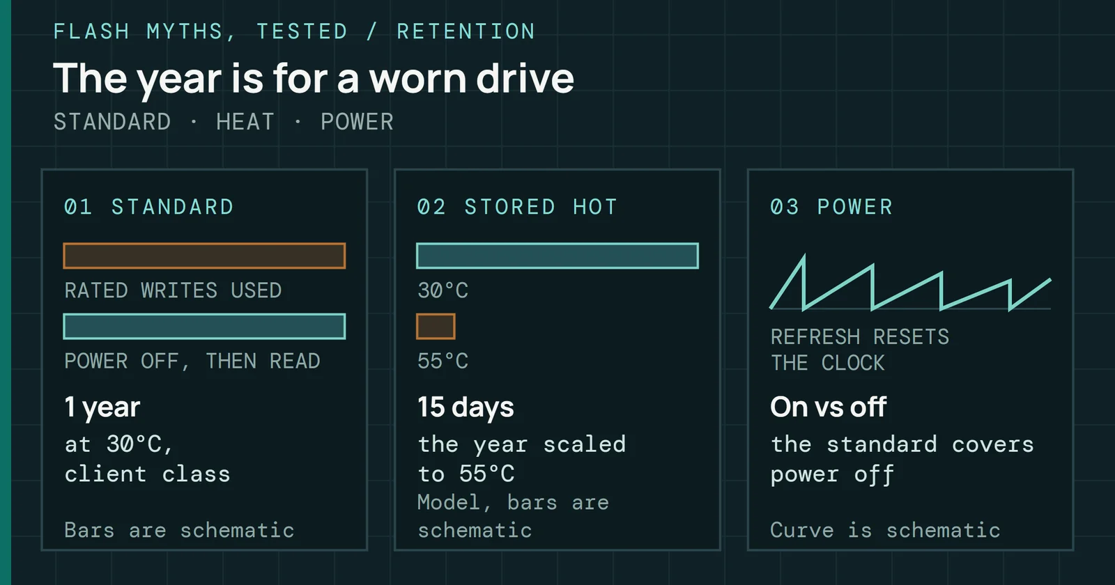
Retention requirements depend on the drive class. A JEDEC-hosted presentation summarizes JESD218 as requiring three months of power-off retention at 40°C for the enterprise class once the drive has used its rated endurance. The client class is summarized as one year at 30°C under the same end-of-life condition. That summary also pairs each class with a powered-use condition for the endurance test, shown with the retention conditions below. It also has retention verified both with a temperature-accelerated mechanism and without acceleration.
| Class | Powered use | Retention unpowered | Uncorrectable bit error ratio |
|---|---|---|---|
| Client | 40°C, 8 hours a day | 1 year at 30°C | 10⁻¹⁵ |
| Enterprise | 55°C, 24 hours a day | 3 months at 40°C | 10⁻¹⁶ |
Temperature acceleration
Charge loss speeds up with temperature, following ArrheniusThe Arrhenius equation relates temperature to the speed of charge loss, so a short bake at high temperature stands in for a long time at normal temperature. kinetics, the same relationship that governs chemical reaction rates and oxide degradation throughout semiconductor physics. For NAND, the practical result is that data retention time drops about 4x for every 10°C increase in storage temperature near room temperature, using the 1.1eV activation energy JEDEC applies. Take the client class’s one year of retention at 30°C. At 40°C, the enterprise class’s temperature, 1.1eV gives an acceleration of about 3.8x, so the same charge loss arrives in about three months, which matches the enterprise class’s three months at 40°C. The shorter time follows from the activation energy and says nothing about a defect.
1.1eV is a qualification convention. Charge-trap retention changes mechanism with temperature, so real activation energies vary, and measurements on 3D charge-trap NAND found about 1.04eV (1.01 to 1.08eV, from a fit that used one value for all temperatures and wear levels). Standards also require a room-temperature check alongside the accelerated one.
Data retention: error rates are not static
Heat shortens retention by orders of magnitude
Charge-loss acceleration against storage temperature, log scale
Figure 8.10 plots the acceleration factor against storage temperature for both activation energies. The two curves are close, and the measured value is slightly gentler. That gap matters when a bake result is converted into storage time.
Refresh, bake tests and power-off failures
Firmware compensates with background data refresh. The controller scans blocks, checks RBER, and rewrites data that is approaching ECC limits with fresh charge levels, which resets the retention clock at a small cost to the P/E budget. Part 7 covers how refresh is scheduled and what it costs.
Arrhenius is also the math behind bake testing. A bake holds a drive at an elevated temperature for a controlled period to accelerate charge loss. A drive baked at 70°C for 24 hours accumulates retention age roughly equivalent to nine months of storage at 25°C using the 1.1eV activation energy and Arrhenius form, a figure computed for this guide, or about six and a half months using the 1.04eV measured on 3D charge-trap parts. That lets retention failure patterns surface in a test session rather than a field deployment.
A drive can show data integrity problems after an extended power-off period, such as seasonal storage, equipment in transit, or spare inventory aging on a shelf. Retention-related RBER is a sensible first mechanism to check. Standard SMART data has no power-off timer, so infer the duration from host logs or shipping records, and combine it with an estimate of the ambient temperature to get the input for the Arrhenius calculation. The output tells the engineer whether observed error rates match the expected retention age, or indicate degradation beyond what the cell type’s retention specification should produce.
Die-level parity: the backstop when ECC runs out
ECC corrects errors at the bit level. Die-level parity covers failures beyond what ECC alone can fix, from a single uncorrectable page up to complete die loss. Micron calls its internal exclusive-OR (XOR) parity scheme RAIN (Redundant Array of Independent NAND), and many SSDs, client and enterprise alike, add some form of die-level parity as a fault-tolerance layer beyond ECC.
Parity data is distributed across multiple dies or channels, entirely within the SSD. If a single NAND die fails completely, whether from a manufacturing defect, a block retirement cascade or sudden electrical damage, the parity on the remaining dies allows full reconstruction of the lost content.
Stripe width, the number of data dies protected by each parity set, determines both fault-tolerance scope and rebuild duration. Published designs use one parity member per stripe, with data-to-parity ratios such as 7:1, 15:1 and 127:1. When each member sits on a different die, one failed die costs each stripe one member.
Die-level parity: the backstop when ECC runs out
One parity member lets a stripe survive a failed die
Eight channels, two dies each, one 7:1 stripe
Figure 8.11 shows one stripe of an eight-channel drive in the 7:1 shape. A complete die-loss rebuild must read every stripe that held data on the failed die, and compute the missing content from the remaining stripe members by XOR. How long that takes depends on the design, and vendors rarely publish it.
Parity consumes capacity and adds write overhead, because the controller must compute and write parity alongside the data. Enterprise drives absorb this overhead in their overprovisioning (OP). Consumer drives vary. Some drives, such as Micron’s, implement RAINRAIN adds parity across dies, much like RAID across drives, so the data from a failed page or even a whole die can be rebuilt. and offer SMART reporting for it, while others rely on ECC and the spare block pool. At small capacities, parity takes a larger share of raw NAND, and the extra die it needs is harder to absorb in unit cost.
In many designs the drive keeps serving host I/O during rebuild. Reads that target pages that lived on the failed die slow down, because each one needs several reads plus an XOR across the surviving stripe members instead of one direct page access. A drive showing elevated tail latency scattered across its LBA range, while a vendor diagnostic log identifies a single die as failed or retired, is consistent with a rebuild.
ECC exhaustion: how failure progresses
Understanding how ECC failure unfolds step by step changes how you interpret symptoms at the host. Firmware manages a graded response as per-block error rates climb toward the limit of the decoder, and each stage has its own observable signature.
ECC exhaustion: how failure progresses
Failure arrives in five stages, and only the last reaches the host
Firmware action and observable symptom at each stage
Figure 8.12 lists the five stages in order. Stage one is elevated RBER. As a block accumulates P/E cycles or retention age, the voltage distributions broaden. Standard reads return more raw bit errors than before but still within what ECC can correct, so the drive functions normally. Potentially slower reads on affected pages are the only sign, because the LDPC decoder is working harder and may be running additional iterations.
When RBER exceeds the standard correction budget, the firmware attempts read retry. Threshold scanning may recover the page at the cost of latency, producing a latency spike where there was previously a single read. If retry succeeds, firmware moves the data to a healthier block and flags the source block for evaluation or retirement.
If retry, soft-decision decoding and die-level parity recovery, where present, all fail, the firmware has reached ECC exhaustionECC exhaustion is the order of recovery steps as errors grow: normal decode, read retry, soft decode, die-level parity, and finally an uncorrectable error. on that location. The read cannot be completed with confidence, and well-implemented firmware returns an error to the host rather than passing along data it cannot trust.
Two stages matter most for diagnosis. During the retry stage the reads still succeed and only the latency changes, so a latency spike on a fixed range of addresses with Media and Data Integrity Errors still at zero is the retry signature. At the last stage the counters finally move.
An early warning inside this sequence is RBER that settles at a higher baseline and stays there. On a healthy block, RBER drops back after read retry tuning or a data refresh. RBER that holds a new floor, higher than the drive’s initial operating level and unresponsive to threshold adjustments, indicates oxide degradation serious enough that the broadening is structural rather than recoverable. A block or region showing this signal is nearing the end of its service life. Only drive-internal or vendor logs show RBER directly.
NVMe protection information: end-to-end data integrity
ECC protects data on the NAND medium. It does not protect data in transit between the drive and the host. A bit flip in the PCIe interconnect, a memory error in the host DRAM buffer, or a firmware bug corrupting a direct memory access (DMA) transfer could deliver incorrect data to the application even if the NAND itself was read perfectly. NVMe Protection Information (PI)NVMe Protection Information attaches a checksum and tag to each block so corruption between host and media can be detected end to end. closes this gap.
NVMe PI adds a metadata block to each logical block. It contains a guard field, a cyclic redundancy check (CRC) over the data (CRC-16 in the base specification, with longer guard CRCs in newer revisions), plus reference tags that verify data identity across the full path from host to NAND and back. When PI is enabled, the host writes data with a computed CRC over the data buffer. The controller verifies the CRC on the way in, keeps the guard field with the data, where in the NAND is a firmware choice, and recomputes and validates the CRC during reads. Corruption anywhere in the protected path produces a CRC mismatch at the next checking point, with very high probability, rather than passing silently to the application.
NVMe protection information: end-to-end data integrity
PI checks the data at every hop between host and NAND
One write and read, five checking points
Figure 8.13 marks the checking points on one write and read. The host driver computes the CRC, the controller checks it on the way in and again before returning data, and the host checks it last. A fault at any hop shows up as a mismatch at the next check.
PI runs only when the host turns it on. Underneath it, some enterprise drives add checks of their own. A 2014 Micron description in Data Center Knowledge has the controller embed the host LBA with the data it writes to NAND and check it on the way back, and add memory-protection ECC (MPECC) as the data enters the drive’s DRAM, coverage that then follows the data through the drive. Both are separate from the NAND ECC this part describes.
Three PI types address different use cases, summarized in the table.
| PI type | Reference tag | Use case |
|---|---|---|
| Type 1 | Carries the logical block address (LBA), so it catches corruption and misdirected writes, where correct data lands at the wrong LBA | The general case |
| Type 2 | Checked against a starting value the host supplies in each command, not the LBA | Software that manages its own block address translation, such as a database engine or hypervisor, and data that moves between LBA ranges |
| Type 3 | Not checked, the CRC guard field alone protects the data | Intermediate layers that remap addresses in ways that break Type 1 or Type 2 tag matching |
The Guard field is a CRC over the data in that block, and the Reference Tag ties the block to its address, so an older version of the same LBA still carries a valid CRC and the right tag and passes every PI check. PI therefore catches corrupted data and data returned from the wrong address and misses a drive that returns the previous version. That failure needs host-side versions or checksums stored apart from the data, as Part 6 describes.
PI needs support from the host driver, any host bus adapter (HBA), RAID card or fabric in the path, and the SSD firmware. A system with PI-capable drives that does not configure PI at the host driver and HBA layer delivers no end-to-end protection. The CRC is not computed on the host side, so corruption in the host buffer is invisible to both ends. PI is used mainly in enterprise NVMe deployments, where the full stack from application to drive can be configured to participate. For deployments where silent data corruption is the failure mode that matters most, PI is the standard NVMe mechanism that checks data across the full path from host memory to NAND and back, catching errors ECC alone would miss, except stale data.
In the field: what ECC failure looks like from the host
A field engineer or support technician has no direct view of internal RBER or per-block wear, and sees retry activity only through vendor-specific logs or Open Compute Project (OCP) telemetry, the logs covered in Micron’s SSD resiliency post. The technician sees what the NVMe interface surfaces.
When ECC exhaustion produces an uncorrectable error, the drive returns a command completion with a non-zero status field. The common case is a media and data integrity error, Status Code Type 2h with Status Code 81h (Unrecovered Read Error). It means the drive attempted to read a page, applied error correction, attempted read retry, and could not recover the data with acceptable confidence. The Do Not Retry (DNR) bit, defined in the NVMe base specification in the Status field of the completion entry signals whether the host should try the command again or treat it as a permanent failure. Operating system logs capture these events, with detail that varies by operating system and storage driver. Linux kernel logs show NVMe I/O error entries with status codes and the affected LBA range, and the Windows Event Log surfaces storage errors through the disk subsystem. In both cases the entry identifies the failed command and address range and says nothing about the physical NAND location or the internal state behind the failure.
Telling a media failure, an interface failure and a firmware fault apart requires cross-referencing several data sources. A media failure typically shows a stable LBA range, with the same logical addresses failing repeatedly across multiple read attempts. Interface failures such as link instability or a worn connector tend to produce errors at different LBAs on each attempt, often alongside other interface-level errors, such as Advanced Error Reporting (AER) receiver or replay errors and link retraining events in the kernel log. A firmware fault may produce unusual status codes that do not map cleanly to media or interface categories, or it may surface as a command timeout rather than an error completion.
In the field: what ECC failure looks like from the host
Failing addresses and link errors sort the three failure types
First-pass checks from the host
Figure 8.14 turns those checks into a first-pass tree. Start with the repeat pattern of failing LBAs, then look for interface errors, and treat what is left as a firmware candidate. Ordering the checks is all the tree does, and a vendor diagnostic still has the last word.
Before opening a support ticket or escalating a drive for replacement, collect the following from the NVMe SMART / Health Information log and error log. This table is the series reference for the fields, and other parts link here.
| Field | What it shows | Why it matters |
|---|---|---|
| Available Spare | Percentage of reserved block pool remaining | The vendor sets the warning threshold, and firmware behavior changes as the value nears zero |
| Available Spare Threshold | Manufacturer-set floor before critical warning triggers | Compare against Available Spare to assess proximity to the threshold |
| Percentage Used | Vendor wear estimate (100% = predicted NVM endurance consumed) | Contextualizes all other wear indicators. Above 100% means operating past rated endurance |
| Media and Data Integrity Errors | Count of unrecovered data integrity errors, such as uncorrectable ECC, CRC failure or LBA tag mismatch | Any non-zero value warrants investigation. Rate of change matters more than absolute count |
| Number of Error Information Log Entries | Lifetime count of error log entries, all causes | Pull the full log to see error types and affected LBA ranges |
| Unsafe Shutdowns | Power loss events without graceful shutdown | High counts can point to mapping table inconsistency on drives without power loss protection |
| Power On Hours | Total operational time | Establishes wear rate context: Data Units Written divided by Power On Hours |
| Data Units Written | Lifetime host writes in 512,000-byte units | Compare against rated terabytes written (TBW)Terabytes written is the total host data a manufacturer rates a drive to absorb over its life under the warranty conditions. to assess the remaining endurance budget |
| Critical Warning | Aggregate status byte for drive-level conditions | Any non-zero value indicates the controller has flagged a condition requiring attention |
This is the minimum evidence set for a storage incident. Without it, telling a wear-related ECC failure, an interface failure and a firmware fault apart is guesswork. With it, the failure category is usually clear within the first pass.
What ECC hands to performance and endurance
The headroom ECC leaves is spent as a drive ages, and the first place it shows is speed. Reads on aged data slow before any counter moves, so a drive that still reports clean health can already be paying for retries and relocations in every read.
What ECC hands to performance and endurance
Error Correction & Integrity feeds one later part.
Arrows run to the parts that build on this one.
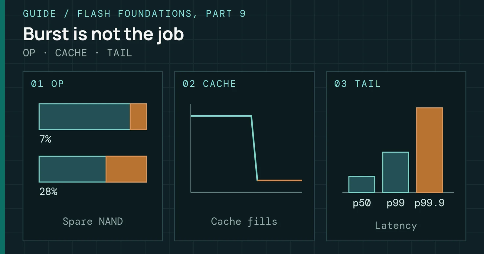
Part 9 picks up from there with the performance side of the same budget. It starts with the spare capacity that gives the controller room to work, then follows how burst and sustained numbers, latency percentiles and endurance ratings change once that room and the ECC headroom run down. Those ratings assume a specific ECC correction budget over the drive’s rated life, and that part asks whether a deployed drive delivers them.
Sources
Primary is the original paper, standard or datasheet. Secondary is a review, a vendor summary or a news report. Measured is my own test data.
Show all 34 sources, 26 primary
- PrimaryError Detecting and Error Correcting CodesBell System Technical Journal, 1950open copy
- PrimaryA Recursive Approach to Low Complexity CodesIEEE Transactions on Information Theory, 1981
- PrimaryGood Error-Correcting Codes Based on Very Sparse Matricesmathe2.uni-bayreuth.de, 1999open copy
- PrimaryMicron TN-29-19, NAND Flash 101 (Rev. B, 2010)Micron Technology, Inc., 2010
- PrimarySF-2200 & SF-2100 Client SSD ProcessorsSandForce, 2011
- PrimarySATA Solid-State Drive Controller Datasheet2014
- PrimaryRead disturb effect determination2015
- PrimaryJESD218B Solid-State Drive (SSD) Requirements and Endurance Test Method (Revision of JESD218A, February 2011)JEDEC Solid State Technology Association, 2016
- PrimaryNAND Flash Media Management AlgorithmsFMS, 2016
- PrimaryController Technologies for Managing 3D NAND Flash MemoriesFMS, 2017
- PrimaryError Characterization, Mitigation, and Recovery in Flash-Memory-Based Solid-State DrivesProceedings of the IEEE, 2017open copy
- PrimaryBeLDPC: Bit Errors Aware Adaptive Rate LDPCDesign, Automation and Test in Europe (DATE) 2020, 2020
- PrimaryNVM Express Base Specification, Revision 2.0NVM Express, Inc., 2021
- PrimaryRead Reference Calibration and Tracking for Non-Volatile Flash MemoriesElectronics 10(18):2306, 2021
- PrimaryReducing Solid-State Drive Read Latency by Optimizing Read-Retry (ASPLOS 2021, arXiv:2104.09611)arXiv, 2021open copy
- PrimaryThe Application of ECC/DSP to Flash Memory (white paper)documents.westerndigital.com, 2021
- PrimaryNVM Express Base Specification, Revision 2.1NVM Express, Inc., 2024
- PrimaryInternational Roadmap for Devices and Systems 2026: Mass Data StorageIEEE IRDS, 2026
- PrimaryAdaptive Read Thresholds for NAND Flashengineering.purdue.edu
- PrimaryHeatWatch: Improving 3D NAND Flash Memory Device Reliability by Exploiting Self-Recovery and Temperature Awareness
- PrimaryImproving 3D NAND Flash Memory Lifetime by Tolerating Early Retention Loss and Process Variation (Luo et al., SIGMETRICS 2018; arXiv:1807.05140)arXivopen copy
- PrimaryJEDEC SSD Specifications Explained: JESD218 and JESD219 (Alvin Cox, Seagate)JEDEC
- PrimaryNAND Flash Media Management Through RAINMicron Technology technical marketing brief
- PrimaryNVM Express Base Specification, Revision 1.4cNVM Express
- PrimaryWhat Types of ECC Should Be Used on Flash Memory? (AN99200)skyhighmemory.com
- PrimaryWorking to revolutionize SSD resiliency with shift-left approachmicron.com
- SecondaryError Correction Codes in NAND Flash MemoryThe University of Texas at Austin (master's report), 2015
- SecondarySoft-Decoding in LDPC based SSD ControllersEE Times, 2015
- SecondarySolid-State-Drives (SSDs) ModelingSpringer, 2017
- SecondaryArchitectural Techniques for Improving NAND Flash Memory ReliabilityCarnegie Mellon University (PhD thesis), 2018
- SecondaryResearch on 3D TLC NAND flash reliability from the perspective of threshold voltage distributionMicroelectronics Reliability, 2020
- SecondaryChannel and Source Coding for Non-Volatile
- SecondaryIntroducing Low-Density Parity-Check Codes (Sarah Johnson)ACoRN Spring School lecture notes, version 1.1
- SecondaryNAND Error-correction Code — The Linux Kernel documentationkernel.org