Flash is analog. A cell does not store a one or a zero. It stores charge, and charge drifts with time, temperature, and wear. Every firmware system in this series is a response to that fact.
Flash Foundations
Flash Foundations, Part 2: The Physics of Flash
See how stored charge becomes data, and why reading it gets harder as cells become denser.
On this page 17 sections
Part 1 set the external limits. They cover standards, protocols, form factors, and drive validation. This part is the physics those limits sit on, down to a single cell.
Electron traps and voltage distributions are why the raw bit error rateRaw bit error rate is the fraction of bits read from the NAND that are wrong before error correction is applied. (RBER) rises with wear, why read retryRead retry rereads a failed page with the read reference voltages shifted, trying a table of offsets until the data decodes. exists, and why quad-level cell (QLC) flash asks far more of the error correction codeError-correcting codes add parity bits to each block of data so the controller can find and fix bit errors on read. (ECC) engine than triple-level cell (TLC) flash. A premature-wear complaint traces back to how the cell holds a bit as charge, why that charge spreads and drifts, and why each added bit costs enduranceEach added bit per cell halves the spacing between voltage levels, which raises capacity and lowers the number of program/erase cycles the cell survives..
What flash actually stores in the cell
A NAND cell is a transistor with a floating gate. The gate is a conductive layer sealed in oxide, between the control gate above and the silicon channel below. This design remains the original architecture and the clearest way to learn the physics. Kahng and Sze introduced the idea in a 1967 floating-gate memory device at Bell Labs. Most modern 3D NAND stores charge in silicon nitride instead of polysilicon. Programming still works by tunneling, and the charge-trap section below covers why the material changed.
Apply enough voltage, and electrons tunnel through the oxide onto the floating gate. They stay when power is removed, which is non-volatility. Erase reverses the trip, pulling them off again and returning the cell to a low Vt, usually below zero.
What flash actually stores in the cell
Charge on the floating gate raises the threshold voltage
A floating-gate cell, then the two Vt states a read tells apart
Figure 2.1 shows the stack on top and what a read asks of it below. Trapped electrons raise the transistor’s threshold voltageThreshold voltage, Vt, is the gate voltage at which a flash cell starts to conduct. The stored charge shifts it, and the controller reads data from it. (Vt), the voltage needed to turn it on. A charged cell needs more voltage to conduct. An empty cell conducts more easily. A read asks whether current flows at one reference voltage (Vref), and that yes-or-no answer is one bit.
Each state in the lower panel is a bell-shaped population, because every cell ends up at a slightly different Vt. A read reference sits in the gap between the populations. That gap is the margin, and every later section in this part spends it.
Threshold voltage is an analog measurement of the stored charge, and that charge varies from cell to cell. Oxide thickness varies. Temperature moves charge. Time lets it leak. Each of those pushes Vt off its intended mark.
How electrons cross the oxide by Fowler-Nordheim tunneling
Electrons enter and leave the floating gate by Fowler-Nordheim tunnelingFowler-Nordheim tunneling is the quantum effect that lets electrons pass through the tunnel oxide when a strong electric field thins the barrier.. That mechanism is why NAND wears, why oxide damage adds up, and why the program/erase (P/E)A program/erase cycle is one write of a block followed by its erase. Each cycle wears the oxide, and the cell type sets how many cycles it tolerates. limit tracks real oxide damage rather than an arbitrary number.
Classically, a particle cannot cross a barrier taller than its energy. Quantum mechanics gives it a probability, set mostly by how thick the barrier is and how strong the field is. Lenzlinger and Snow measured exactly this for electrons tunneling into thermally grown silicon dioxide in 1969. Tunneling oxide in a floating-gate cellA floating-gate cell stores data as charge on a conductive polysilicon layer that is fully insulated, so the charge stays after power is removed. ran from about 10nm down to about 7nm by the last planar nodes. Much thinner than that and stress-induced leakage current (SILC) lets the cell lose its stored charge. At program fields, on the order of 10MV/cm, electrons from the channel have enough tunneling probability to reach the floating gate.
Programming puts a high positive voltage on the control gate, typically about 15 to 25V, depending on the design, applied as a staircase of short pulses. A 1995 32Mb planar part stepped from 15.5V up to 20V. That field drives Fowler-Nordheim injection. Electrons leave the channel, cross the oxide, and collect on the floating gate. More electrons, higher Vt.
How electrons cross the oxide by Fowler-Nordheim tunneling
A tilted oxide band is thin enough for electrons to cross
Electron energy across the channel, tunnel oxide and floating gate
Figure 2.2 plots electron energy across the channel, the tunnel oxideThe tunnel oxide is the thin insulating layer between the channel and the charge-storage layer. Electrons cross it during program and erase, and it wears out. and the floating gate. Bias tilts the oxide’s conduction band, so the barrier an electron has to cross shrinks to a thin triangle. Under program bias the electron crosses from channel to gate. Under erase bias the tilt reverses and it crosses back.
Erase flips the polarity. In planar NAND, the whole well rises to about 20V while every wordline in the block sits at 0V, so no negative voltage is needed and the field pulls the electrons back out. Electrons leave the floating gate and Vt falls to the erased state, usually below zero. Erase uses the same mechanism with the sign reversed. Many 3D NAND designs erase differently, as the erase section shows. Oxide takes damage whichever way the electrons travel, so P/E budgets count both.
Where 20V comes from
A NAND die runs from a low supply and needs roughly 15 to 25V on a wordline. It builds the difference on the die with charge pumps. A pump moves charge through a chain of capacitors, and each stage adds about one supply voltage, so N stages give roughly N times the supply, less losses (Dickson’s on-chip voltage multiplier is the classic version). Real pumps fall short of the ideal. A doubler-based pump design can reach more than 25V from a 2.5V supply, with an efficiency as high as 20 to 30% when the load stays in range. At that efficiency most of the input power is lost as heat.
NOR programs a different way
A NOR cell does not tunnel to program. It uses channel hot-electron injectionChannel hot-electron injection programs a cell by accelerating electrons along the channel until some gain enough energy to jump the oxide. NOR flash uses it., with a high voltage on the control gate, a bias on the drain, and the source grounded. Only the few carriers that gain enough energy near the drain climb over the oxide barrier onto the floating gate. Hot-electron injection draws real current from every cell it programs, which caps how many cells can program at once. Tunneling draws almost no current, which is why NAND can program a whole page in parallel.
Programming a cell into a narrow window
You cannot program a cell into one of 8 or 16 states with one big pulse. Too much voltage and it overshoots, and you cannot pull charge back from one cell without erasing the whole block. Incremental step-pulse programmingIncremental step pulse programming raises the program voltage a small step with every pulse and checks the cell between pulses, so charge lands precisely. (ISPP, Suh and colleagues) is the workaround. It pulses, senses Vt, steps up a little if the cell is short of the window, senses again, and stops when it reaches the window.
Two things set how tightly a programmed state can land. First, once a cell is programming steadily, each pulse raises its Vt by about the size of the step, so the step size sets how wide the final distribution is. Second, electrons arrive one at a time, at random. A step that moves Vt by ΔV through a total capacitance C delivers about CΔV/q electrons, and counting statistics make the delivered number uncertain by its square root. That leaves a spread of roughly √(qΔV/C) in the final voltage even with a perfect circuit, a floor that matters more as cells shrink and states pack closer.
Programming a cell into a narrow window
Pulse, verify, step, and stop inside the window
You cannot pull charge back from one cell, so an overshoot means erasing the block
A single-level cell (SLC) has two states and wide margins, so it needs only a handful of pulses. TLC has eight states and needs more pulses to reach each target without overshooting. QLC has sixteen states with an illustrative fresh gap of 50 to 80mV between them, the space left between states that each occupy a few hundred mV. The table in the SLC-to-QLC section gives the estimate. With that little room, QLC needs finer verify and many more pulses. Each cycle wears the oxide in much the same way for every cell type, but QLC has far less margin to lose, so the same wear ends its life sooner.
The charge trap behind modern 3D NAND
NAND physics is usually taught with the floating-gate model, and the tunneling description is right. Most 3D NAND in production, though, stores charge in silicon nitride instead. Samsung V-NAND, Kioxia BiCS, current Micron 3D NAND, and SK hynix 4D NAND all use nitride. Micron’s 176-layer and SK hynix’s 238-layer NAND are also charge-trap. Solidigm is the main exception. Its high-capacity drives use floating-gate NAND, and its PLC NAND will too. One big reason is what a conductor does, versus an insulator, when the oxide inevitably defects.
In a floating-gate cell, electrons sit on a continuous polysilicon sheet, so charge spreads across the whole conductor. A pinhole anywhere in the tunneling oxide gives the entire stored charge a leak, and one defect can lose all of it. At the feature sizes planar NAND reached before scaling stopped, that became a reliability wall, and it is one of the reasons the industry went vertical.
Silicon nitride is an insulator. Trapped electrons mostly stay at the defect sites that captured them, so a pinhole leaks only the nearby sites. Everything else in the nitride keeps its charge. Charge trap tolerates local oxide damage because the stored charge cannot run to the leak.
The charge trap behind modern 3D NAND
A pinhole drains a floating gate but only part of a charge trap
Both cells with the same defect in the tunnel oxide
Figure 2.4 puts the same pinhole in both cells. Every electron on the floating-gate sheet on the left can drain through it, while only the trap beside the defect loses its charge in the charge-trap cell on the right. That tolerance matters when you deposit hundreds of layers and cannot keep oxide as uniform as a planar process can.
Isolated storage sites were first explored in nanocrystal memories, where each nanocrystal holds its own small share of the charge. Tiwari and colleagues at IBM stored electrons in silicon nanocrystals about 5nm across, and trade press reported that Freescale had proven a 24-Mbit nanocrystal array in 90nm processing. Nanocrystals did not scale, though. They gave a smaller Vt shift (Tiwari reported 0.2 to 0.4V) and left percolation paths between source and drain. A NAND-type MONOS memory built at a 63nm process put a nitride between tunnel and blocking oxides and showed negligible capacitive interference between cells. Floating gate keeps a strength of its own. An electron leaving it has to climb a barrier of about 3.2eV, and floating-gate cells are known for their data retention.
Less coupling is the other gain. A floating gate is a conductor, so a neighbor’s stored charge couples into it and shifts Vt with no new program pulse. Charge trap does couple less, but the nitride is not the main reason. In 3D cells much of the drop comes from the control gate wrapping around each cell, which shields the cell from its neighbors. Goda’s review of 3D floating-gate cells reports good shielding of cell-to-cell interference even though the storage layer is conductive.
Charge trap has its own drift, though. Nitride runs unbroken down the string, so trapped charge can migrate sideways into the gaps between cells, a retention-loss mechanism vendors design around that acts over a long time and depends on what the neighbors hold. A separate effect, early retention loss in charge-trap cells, shows up within seconds and hours of programming and is steep at first. In a vertical string with a wordline pitch of only 43 to 58nm in measured production dies, those two effects set how tightly the layers can pack. Part 4 lists the measured pitches.
What the round channel changes
A vertical charge-trap cellA charge-trap cell holds electrons in discrete traps in an insulating nitride layer instead of on a conductive gate, so one defect cannot drain the whole charge. wraps its gate around the channel, and that geometry has side effects. For the same dielectric thicknesses, in the modeled geometry the field at the tunnel oxide peaks at about three times the planar value, while the field across the blocking oxide is lower. That helps programming and relieves erase saturation, where electrons from the gate leak back in during erase. That shared nitride film is also the lateral path described above. Simulations of TCAT devices find that it dominates over vertical loss, that its share grows as the gate gets shorter, and that heat speeds it up. Samsung’s TCAT process shapes the charge-trap layer into a biconcave profile, which reduces the spreading. Even reading costs a little. Charge loss scales with cumulative sensing time, and short sensing times keep it small.
A ferroelectric FET stores its bit differently again, in the polarization of its gate insulator. The Beyond NAND guide covers it.
Erase: pulling electrons out versus pushing holes in
Planar NAND raises the shared p-well under the array, and that well is an endless supply of holes. Toshiba’s BiCS strings stand on an n+ source line with no p-type body to draw from, so they used gate-induced drain leakage (GIDL) eraseGate-induced drain leakage erase raises the channel voltage at the end of a string until holes are generated that erase the cells above., as an overview of 3D NAND integration describes for both schemes. Samsung’s TCAT stood its pillars on the p-type substrate and erased through the body, planar style. CMOS-under-array designs, which put the periphery beneath the array, typically erase by GIDL as well.
GIDL bias puts a high voltage on the bitline and source line and holds the select gates below it. Band-to-band tunneling at each string end generates electron-hole pairs, and the holes charge the string body. Holes then tunnel from the body into the nitride at every wordline to neutralize trapped electrons, with no sweep of the substrate.
Erase: pulling electrons out versus pushing holes in
Planar erase pulls electrons out. String erase pushes holes in.
A well under the cell versus gate-induced drain leakage at the string ends
Figure 2.5 sets the two paths side by side. On the left path the well is the sink for electrons, and on the right path the string ends are the source of holes, with the wordlines at 0V. Both methods end in the same place, a block with every cell back at the erased Vt, and both put stress on the oxide.
GIDL has two faces
In an inhibited string the channel is boosted high, and the select transistor beside the first wordline is off with a large voltage across its edge. GIDL there makes electron-hole pairs, and the electrons arrive hot. Some of them program the neighboring wordline when they should not. It is a known program-disturb mechanism in planar NAND, and dummy wordlines shield the edge cells. 3D NAND puts the same physics to work. Band-to-band tunneling disturbs an edge wordline and also makes the holes that erase the block. Part 4 covers why the cells at the ends of a string behave differently from the ones in the middle.
Random telegraph noise and the flickering worn cell
A floating gate holds its charge as a shared pool, so at larger nodes a small loss looks like smooth Vt drift. Single traps in the polysilicon channel of 3D NAND, mostly at grain boundaries, and in the tunnel oxide capture and release carriers. When one flips, cell current jumps and the sensed Vt steps, then may step back. Engineers call this random telegraph noise, or RTNRandom telegraph noise is a small threshold-voltage jump that appears when one electron is repeatedly captured and released by a single trap near the channel.. A cell’s Vt is not stable between reads.
Fresh NAND has fewer oxide traps, so RTN is quieter. Wear can add traps, though 3D measurements show only a modest rise in RTN with cycling (one study found a stronger dependence). Floating-gate NAND had RTN too, and for 3D NAND another large source comes from traps at the grain boundaries of the polysilicon channel. Toshiba’s BiCS used a thin polysilicon channel, which removes the defective central region of a thick one.
Random telegraph noise and the flickering worn cell
A floating gate drifts smoothly; a single trap steps the sensed Vt
Same tunneling oxide, different storage, different failure shape
In the left panel the floating gate drifts smoothly, and in the right panel one trap flips and steps the sensed Vt. A cell hit by RTN reads correctly most of the time and fails now and then, with no repeatable error at a fixed Vref. Read retry can pass on one attempt and fail on the next because the Vt actually moved, so a read that passes in testing can still fail in service. On worn drives RTN can add to tail latency, because the retry loop has to keep going until a pass is confident. Add many traps together and their separate telegraph signals blur into a smooth 1/f noise spectrum.
From one bit to four: the SLC-to-QLC progression
The original flash cells stored one bit, charged or not, and that design is SLC, with wide margins, easy reads and the longest oxide life of any cell type. Density is the cost. One bit per cell means low-capacity dies at a high cost per gigabyte, so the industry needed more bits on the same die.
Multi-level cell (MLC) flash stores two bits by distinguishing four voltage levels. Same transistor, four states instead of two. Margins shrink. Reads need tighter voltage control, endurance drops, and stronger ECC and smarter controllers become necessary. TLC stores three bits across eight levels. Margins shrink again and error rates climb, so the controller leans harder on ECC and firmware.
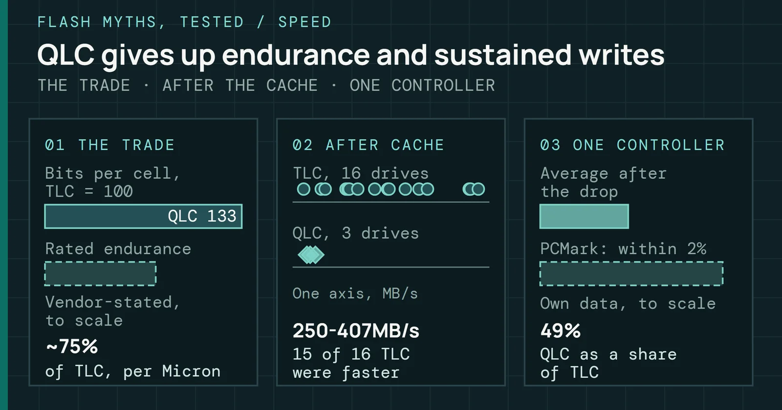
QLC stores four bits across sixteen levels. Its illustrative fresh gap is 50 to 80mV where SLC’s is 1V or more. QLC drives rely on advanced ECC, wear leveling, and read retry to stay readable.
From one bit to four: the SLC-to-QLC progression
More bits per cell means more states in the same Vt range
Same range, more windows, less room for each
Figure 2.7 is the reason. Each bump is one voltage state, and the gaps are the read-reference zones. With the usable Vt range fixed, more windows mean less room in each one. Every added bit doubles the states and halves the room.
The table gives the progression, ending with penta-level cell (PLC)PLC stores five bits per cell using thirty-two voltage levels, which packs more data into the same silicon but leaves very little margin between levels. flash, which has no commercial products yet. Guard bandA guard band is the gap kept between a read reference voltage and the nearest distribution, so ordinary drift does not turn into read errors. is the voltage separation between adjacent threshold distributions. Vendors do not publish Vt margins, and real values vary by die, wordline, and temperature, so the margin values are illustrative estimates. One real anchor is an example in a SanDisk patent: a threshold window from −1.5V to 5V, 6.5V wide, in which each of 16 states “may occupy” 200 to 300mV. Sixteen states of that width fill only part of the window, and the rest is gaps and spare range. The cycle ratings are Lexar Enterprise’s typical figures.
| Cell type | Bits per cell (states) | Fresh gap (mV, illustrative) | End-of-life gap (mV, illustrative) | Typical rated P/E cycles (Lexar) | Status |
|---|---|---|---|---|---|
| SLC | 1 (2) | 1,000+ | 600+ | 50,000–100,000 | Production |
| MLC | 2 (4) | 300–500 | 150+ | 3,000–10,000 | Niche production |
| TLC | 3 (8) | 100–200 | 50–80 | 1,000–3,000 | Production (dominant) |
| QLC | 4 (16) | 50–80 | 15–25 | 150–1,000 | Production |
| PLC | 5 (32) | 25–40 (estimated) | Not established | Not established | No commercial products |
P/E values are nominal ratings. Planar NAND lifetime fell from 10,000 cycles at 70nm to about 2,000 at 1X nm, while early 3D MLC was rated far higher, as Luo and colleagues report. The MLC row spans planar nodes. JESD47 qualifies cycling at both room temperature and elevated temperature. In consumer drives, SLC usually appears as an SLC cache, a firmware-run mode on TLC or QLC NAND (Part 6 covers the mechanism and Part 9 the behavior). Under some conditions a drive can also bypass the cache and write straight to TLC or QLC. Native SLC still exists in specialty low-latency parts such as Kioxia’s XL-FLASH.
PLC: five bits, thirty-two states
PLC is not yet a mainstream product, and Part 10 looks at what comes next. PLC gains about 25% density over QLC. Its problem is the narrow windows, since 32 states with a gap the table above estimates at 25 to 40mV push ECC to or past current low-density parity-checkLDPC is a code whose decoder passes confidence messages back and forth until the errors resolve. It corrects more errors than BCH, especially with soft input. (LDPC) limits. Kioxia and Western Digital, whose flash business is now Sandisk, both presented PLC work at Flash Memory Summit in 2019, and Solidigm showed a working PLC SSD at Flash Memory Summit in 2022. SK hynix showed a split-cell idea at IEDM in December 2025 that cuts the required state count by about two-thirds, adding structural complexity to win back speed and endurance. The 2019 guess has not come true. Blocks and Files then wrote that initial PLC product might arrive in 2021 or 2022 if development issues were straightforward, and in January 2026 it reported that QLC is made commercially but PLC is not. Treat a PLC launch date as roadmap until a product exists.
Voltage distributions: how wear shows up in the physics
Fresh NAND has clean, separated Vt distributions. A TLC block shows eight tight clusters with guard bands wide enough that a Vref in the middle of each gap is almost always right.
Each tunnel event, program or erase, nicks the oxide. High-energy electrons create trap sites at the silicon-oxide interface and in the oxide bulk. Some recover between cycles, but many stay at operating temperature. Rest time matters. In 3D charge-trap cells, a longer wait between cycles slows the later loss of charge, though it does not cure the errors that come from imprecise programming. After thousands of cycles you can measure the damage. Interface traps hold charge that shifts Vt without a program. Bulk traps leak charge at rest. Trapped charge screens the field in part, but damaged oxide also lets charge through more easily. In planar parts, measured program time falls with wear rather than rising, and Part 3 shows the timing data. Wider distributions and slower erase are the lasting cost.
Voltage distributions: how wear shows up in the physics
Wear widens each state until neighboring tails overlap
Eight TLC states on one Vt axis, fresh and worn
Figure 2.8 shows the result on TLC. Worn states are broader and have shifted. In an illustrative case, a 200mV gap can fall to 80mV or less. A Vref that once split state three from state four now errors on the high tail of three or the low tail of four. Those are raw bit errors, and the silicon is returning the wrong answer.
So RBER rises over life because oxide damage shows up as wider Vt distributions. More block erases mean wider clusters and more raw bit errors. Wear reaches the P/E cycle limit at the count where damaged oxide can no longer hold charge inside the required Vt window for the rated retention time, under the specified ECC. Oxide thickness is its own trade-off. Thinner oxide programs and erases faster at lower voltage, and leaks more at rest. Thicker oxide holds charge longer, and needs more voltage and time.
Firmware answers in two main ways. LDPC corrects what it can on every read. When decode fails, read retry nudges Vref and reads again, looking for a cut that catches fewer tails. As the drive ages, both work harder on distributions that overlap more.
Retention is the time axis. Intact oxide holds charge for years. Damaged oxide leaks faster. Vt drifts even when you stop cycling, and a drive that has been off for a long time can read dirtier on first access because charge has had time to move. Bit Drift Tracer measures the read-speed cost of that in real files at rest, plotted against data age.
Reads disturb the other cells in the block through a different path. Sensing one cell applies a pass voltage to every unselected wordline, which acts as a weak program that worn oxide makes worse. Part 3 owns the mechanism, and Part 7 covers how firmware counts reads and relocates data before ECC runs out.
How heat moves the read and the retention
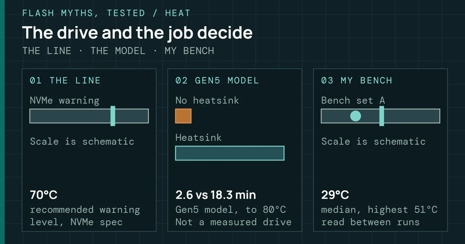
JESD47 qualifies the same rated cycle count at 25°C and again at an elevated temperature between 55°C and 85°C (iST’s JESD47 test-conditions table lists them). Heat costs retention and read margin on worn blocks, and QLC has the least margin to spare. For dense chassis, unventilated M.2 slots, and hot edge boxes, plan for shorter retention and more throttling. Spec sheets give the rated cycle count at those temperatures, but not retention on a worn drive in a hot rack. Heat is not purely a cost, because on 3D charge-trap parts, programming at a higher temperature places the states more tightly and cuts program errors, while storing data hot speeds its charge loss.
Temperature also moves the read, separately from retention. Vt depends on how much charge is stored and on the temperature at which you sense it. Program at one temperature, read at another, and the distribution shifts. On average the direction is consistent. Read colder than you programmed and Vt shifts up. Read hotter and it shifts down. Shift size also varies by state and from cell to cell in 3D arrays. In one published MLC design a cell’s threshold moved by about 1.5mV per degree, roughly 200mV from -40 to 90°C, as wide as the 200 to 300mV that the SanDisk patent above gives each of 16 states. 3D NAND adds a second problem. Its polysilicon channel conducts worse when cold, because grain-boundary traps put barriers in the current path. Cold reads see less cell current and wider Vt spread, and RTN steps grow, because one blocked path matters more when fewer paths remain.
How heat moves the read and the retention
Read colder than programmed and Vt reads higher; hotter, lower
Vt shift of a cell programmed at 25°C, in one published MLC design
Compensation happens in two places. On the die, read and verify levels can shift with temperature, and the bitline bias can rise when cold to offset the lower current. Controllers can also track the best read level themselves, as in dynamic Vt tracking for cross-temperature suppression in 3D TLC. Firmware can also refresh data that was written at a very different temperature. Consumer drives in a stable room rarely notice. Edge, automotive, and industrial boxes that swing between extremes do, and a temperature swing will eat the margin if firmware ignores it. Extended-temperature SKUs exist partly for this reason.
Cell type as a physics constraint: write budget against workload
A cell type should be chosen by its P/E budget against the workload’s write intensity, not by the capacity and price it is sold on.
Cell type as a physics constraint: write budget against workload
Write-heavy logs spend QLC's budget fastest; reads barely spend it
Share of the program and erase budget spent, by cell type and workload
A write-ahead log is a heavy write load. For example, SQLite’s log grows with each commit until a checkpoint, then restarts from the beginning of the file. Under that load, QLC’s small cycle budget goes quickly, while enterprise TLC with more spare area lasts longer. A read-heavy analytics archive writes once and then serves reads. Reads do not spend P/E directly, so that drive can sit at a low cycle count for years, even when the drive is very large. Kioxia announced the LC9, a QLC enterprise SSD, with up to 245.76TB in July 2025, so a single drive can hold hundreds of terabytes. QLC belongs there, because the density is used and the endurance budget stays mostly unspent. A cold archive inverts the question. Retention is the limiting spec, and heat shortens it, as the temperature section explains. Powering the drive on periodically lets background refresh run.
Take a 1TB drive with an illustrative budget of 1,000 cycles per cell, the top of the QLC range above. That is about 1,000TB of NAND writes in total, ignoring spare area. At a WAF of 2, the host can write about 500TB. At a WAF of 5, the host can write only about 200TB. Cells and cycles stay the same, but the budget shrinks as write amplification grows.
Write amplification is the multiplier. Write amplification factorWrite amplification factor is the data written to NAND divided by the data the host wrote. A value of 1 means no extra internal writes. (WAF) is the ratio of actual NAND write volume to host-reported write volume, so it multiplies the P/E cost of every host write. Part 7 defines and measures it. Part 9 owns the selection rules, including how terabytes written (TBW)Terabytes written is the total host data a manufacturer rates a drive to absorb over its life under the warranty conditions. and drive writes per day (DWPD)Drive writes per day is the number of times the full capacity can be written each day for the warranty period, which equals TBW divided by capacity and days. ratings are built, and what they assume.
Wear that runs faster than the writes explain
The usual field mistake is buying QLC for the price and putting it in a write-intensive role. Customers notice when spare is gone or errors show up at what feels like premature end of life. DWPD was the warning. DWPD is the daily write volume a drive can take over its rated life, from P/E budget and usable capacity. Say a QLC drive is rated 0.3 DWPD. It cannot take a full drive write per day and still last its warranty.
On intake for premature wear, cell type is the first question. A drive’s NVMe SMART / Health Information log gives Available Spare, Percentage Used, and Media and Data Integrity Errors. Compare Percentage Used with host writes against the drive’s rated TBW. If wear is faster than the write volume can explain, the next question is WAF. Percentage Used tracks the cycle budget spent, while Available Spare tracks the reserve of spare blocks. A drive can lose spare faster than it spends cycles when blocks fail early, which points at a defect or at heat rather than at the workload, and the temperature section explains how heat eats margin.
Wear that runs faster than the writes explain
Compare wear with writes before blaming the silicon
Two questions, then an outcome
Figure 2.11 reads from the top. If wear matches the writes, the drive is doing what it was rated for. If wear runs ahead and WAF is high, the cause is how the drive is being written, such as too little overprovisioningOverprovisioning is flash capacity held back from the user. The controller uses it as working space for garbage collection, which lowers write amplification. (OP) or no TRIM, which is the territory of Part 7. If wear runs ahead and WAF is normal, the drive is spending its budget as designed, and the budget is too small for the job. Firmware faults sit outside this tree and show up as counters that do not agree with each other. Part 8 covers the error counters.
What the cell physics hands to the cell hierarchy
The SMART Percentage Used value and the error counters are that wear in telemetry, and they are where a premature-wear complaint starts. Because a cell that read fine at a fixed reference can fail later, the controller needs retries and strong error correction before the host sees any data.
What the cell physics hands to the cell hierarchy
The Physics of Flash feeds 2 later parts.
Arrows run to the parts that build on this one.
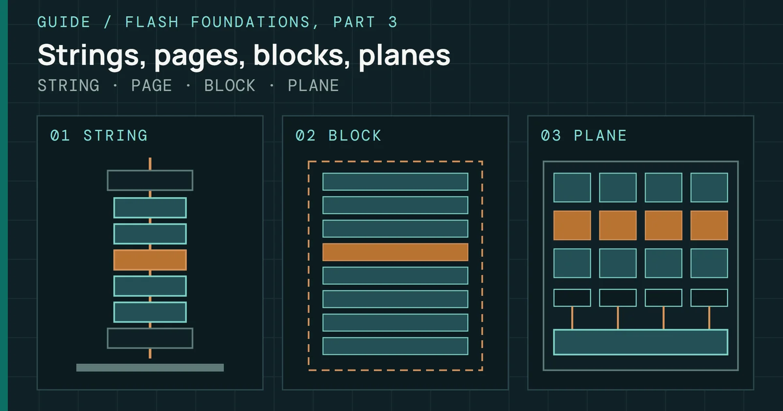
How are cells wired so that a read, a program or an erase reaches one page and leaves the rest alone? Part 3 takes that up. Strings, pages, blocks, planes and dies decide what each operation can touch. Error handling for the physics above is built later, starting with the codes in Part 8.
Sources
Primary is the original paper, standard or datasheet. Secondary is a review, a vendor summary or a news report. Measured is my own test data.
Show all 45 sources, 23 primary
- PrimaryLenzlinger and Snow 1969, Fowler-Nordheim Tunneling into Thermally Grown SiO2 (Crossref record)Crossref, 1969
- PrimaryOn-chip high-voltage generation in MNOS integrated circuits using an improved voltage multiplier techniqueIEEE (Journal of Solid-State Circuits), 1976
- PrimaryA 3.3 V 32 Mb NAND Flash Memory with Incremental Step Pulse Programming Scheme1995
- PrimaryA silicon nanocrystals based memoryApplied Physics Letters, 1996
- PrimarySingle-Electron Devices and Their ApplicationsProceedings of the IEEE, 1999
- PrimaryCharacterizing Flash Memory:Anomalies, Observations, and ApplicationsMICRO, 2009
- PrimaryInside NAND Flash MemoriesSpringer, 2010
- PrimaryUS8725935B2 - Balanced performance for on-chip folding of non-volatile memoriesGoogle Patents, 2012
- PrimaryArchitectural and Integration Options for 3D NAND Flash MemoriesComputers, 2017
- PrimaryA 128Gb 1-bit/Cell 96-Word-Line-Layer 3D Flash Memory to Improve the Random Read Latency With tProg = 75 μs and tR = 4 μsIEEE Journal of Solid-State Circuits, 2021
- PrimarySolidigm Demonstrates World’s First Penta-Level Cell SSD at Flash Memory SummitSolidigm newsroom, 2022
- PrimaryA novel NAND-type MONOS memory using 63nm process technology for multi-gigabit flash EEPROMsdoi.org
- PrimaryCrossref record: A Floating Gate and Its Application to Memory DevicesCrossref
- PrimaryError Characterization, Mitigation, and Recovery in Flash-Memory-Based Solid-State Drives
- PrimaryFrontgrade UT81NDQ512G8T: 4Tb TLC NAND Flash datasheet
- PrimaryHeatWatch: Improving 3D NAND Flash Memory Device Reliability by Exploiting Self-Recovery and Temperature Awareness
- PrimaryImproving 3D NAND Flash Memory Lifetime by Tolerating Early Retention Loss and Process Variation (Luo et al., SIGMETRICS 2018; arXiv:1807.05140)arXivopen copy
- PrimaryKIOXIA Announces Industry’s First 245.76 TB NVMe SSD Built for the Demands of Generative AI EnvironmentsKIOXIA America, Inc.
- PrimaryMicron Technology, Inc. - Micron Ships World’s First 176-Layer NAND, Delivering A Breakthrough in Flash Memory Performance and Density
- PrimaryPowerEdge: Data Retention Occur with SSD or Nvme Drives Due to Prolonged Power offdell.com
- PrimaryScalable Wordline Shielding Scheme using Dummy Cell beyond 40 nm NAND Flash Memory for Eliminating Abnormal Disturb of Edge Memory Celliopscience.iop.org
- PrimarySK hynix Develops World’s Highest 238-Layer 4D NAND FlashSK hynix Newsroom
- PrimaryWrite-Ahead Loggingsqlite.org
- SecondaryCharge-Trapping Non-Volatile MemoriesSpringer, 2015
- Secondary3D Flash MemoriesSpringer, 2016
- Secondary3D NAND with partial block erase2016
- SecondaryInside Solid State Drives (SSDs), Second EditionSpringer, 2018
- SecondaryiST Non-volatile Memory Reliability test conditions (JESD 47 Table 1a)iST (Integrated Service Technology), 2019
- SecondaryWD and Tosh talk up penta-level cell flashBlocks & Files, 2019
- Secondary3-D NAND Technology Achievements and Future Scaling PerspectivesIEEE Transactions on Electron Devices, 2020
- Secondary4 bits/cell 96 Layer Floating Gate 3D NAND with CMOS under Array Technology and SSDs2020
- SecondaryArchitecture and Process Integration Overview of 3D NAND Flash Technologies (Applied Sciences 11(15) 6703)Applied Sciences, 2021
- SecondaryRecent Progress on 3D NAND Flash TechnologiesElectronics, 2021
- SecondaryMicron Ships the Industry’s First 176-Layer QLC NAND in Volume and Unveils the 2400 PCIe Gen4 Client SSDGlobeNewswire News Room, 2022
- SecondarySemiconductor Memories and SystemsWoodhead Publishing (Elsevier), 2022
- SecondaryThe future of NAND technologySamsung Semiconductor Global, 2023
- SecondaryAdvanced Memory TechnologyRSC, 2024
- SecondaryComparing NAND Flash Technology: SLC, MLC, TLC, and QLC for Industrial ApplicationsLexar Enterprise, 2026
- SecondarySK hynix developing split-cell 5-bit flashBlocks & Files, 2026
- Secondary1971: Reusable semiconductor ROM introduced | The Storage EngineComputer History Museum
- SecondaryEnergy-band engineering for improved charge retention in double floating-gate single-electron memories [single-electron FG]arXiv
- SecondaryFreescale demos 24-Mbit nanocrystal memorySemiconductor Digest
- SecondaryInternational Roadmap for Devices and Systems 2022 Edition: Beyond CMOS and Emerging Materials Integration
- SecondaryNOR Flash Data Retention and Endurance introduction application noteRenesas
- SecondarySK hynix Unveils the Industry’s Most Multilayered 176-Layer 4D NAND FlashSK hynix Newsroom