SSD Benchmarking 201, Part 2: Steady State and Tail Latency

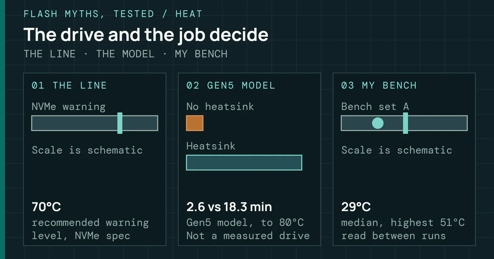
Part 1 ended on a question its job files couldn’t answer: was the drive ready to be measured when the clock started? A flash SSD has no single speed. A fresh drive runs fast for a while and then settles to a level it holds for the rest of its working life, and only that settled level says how it behaves in service. To turn “settled” into a test with limits, SNIA wrote the Solid State Storage Performance Test Specification (PTS).

This part puts my 2016 rounds on a Micron 9100 MAX 2.4TB against that test and then looks at what an average hides. One step in my sweep averaged 0.153ms per read and logged a maximum of 3.3ms for its slowest one. Latency percentilesA latency percentile gives the time within which that share of commands finished. The 99th percentile is the time that 99% of commands beat. fill the space between those two numbers. Iometer only gives them as an estimate from its histogram, and fio reports them directly.

What the SNIA PTS counts as steady state

The introductory series’ part on a repeatable test method covers why a fresh drive needs filling before it’s tested. A PTS run goes further and starts every test from a known state. First comes a purge, by an ATA security erase, an NVMe format, or a vendor tool, which returns the drive as close as it can get to never written, and the report names the method. Workload-independent preconditioning follows, with 128KiB sequential writes over twice the user capacity. After that the test loop serves as its own workload-dependent preconditioning and repeats until the drive settles.

For the test of I/O operations per second (IOPS), that loop is 56 one-minute runs, every pairing of seven read and write mixes with eight random block sizes from 1,024KiB down to 0.5KiB. One pass through all 56 is a round. Rounds repeat until the drive reaches steady stateSteady state is the condition where performance has stopped changing because the drive is full of data and garbage collection runs continuously. or 25 have run. For enterprise drives the PTS recommends four threads at 32 outstanding I/Os each, with the drive’s volatile write cache disabled.

Flash Foundations Part 9 walks through the two-part definition on a real write log. Across a window of the last five rounds, the tracked result’s range must stay under 20% of its average, and a line fitted through those rounds must change by no more than 10% of it.

Which result gets tracked changed between versions. PTS Enterprise version 1.1 tracked one result, 4KiB random writes. Version 2.0 merged the enterprise and client specs and tracks three, adding 64KiB at 65% reads and 1,024KiB random reads, because newer, larger SSDs can be tuned for 4KiB random writes and settle on that result before the others do.

A report carries as much weight as the limits. It needs a convergence plot of every round from the first to the last, a plot of the window rounds against the limits, and a table of the window results. A drive that hasn’t settled by round 25 can keep running or stop there, and a report that stops has to say steady state wasn’t reached.

My 2016 rounds against the rule

My SNIA-style batch file ran one sequential fill and then my 56-spec config 25 times back to back, on my test system with Iometer 1.1.0. It’s the same 2h, 128KiB sequential fill from Part 1, run at a queue depth (QD)IOPS counts commands finished per second. Queue depth is how many commands are outstanding at once, and a drive needs a deeper queue to reach its top IOPS. of 256, and the batch sends its results to a throwaway file. Each round on the 9100 MAX took about 56 minutes. Round 22 started at 20:38:45 on June 20, 2016, and round 23 at 21:35:02, and my workbook keeps rounds 22 to 25.

All 56 specs pass both limits by a wide margin across those four rounds. Version 1.1’s tracked result, 4KiB random writes, ran from 336,992 to 338,321 IOPS around a 337,722 average. That’s a range of 0.4%, and a line fitted through the four rounds moves 0.1%. Both results that version 2.0 added are as flat, with a 0.2% range for 64KiB at 65% reads and 0.3% for 1MiB random reads. My widest range of any spec was 0.5%, at 1MiB with 50% reads, against the PTS limit of under 20%.

How my method differs from the spec

My window differs from the PTS in ways the kept files show. It is four rounds where the spec asks for five, and rounds 1 to 21 aren’t in the workbook, so there is no convergence plot of when the drive settled. The four rounds I kept pass both limits. My batch file starts at the fill with no purge step listed, and the results files don’t record a purge method.

My config departs from the spec twice more. It runs 16 workers at 16 outstanding I/Os, QD256 in total, against the recommended four at 32, and the PTS leaves that choice to the operator as long as the report states it. The PTS asks that its loop order be kept, and mine differs. My config runs block size as the outer loop from 512B up, with read shares from 0% up inside it, while the PTS nests them the other way. Its read mix sits outside, starting at 100% reads, with block size inside from 1,024KiB down. Each one-minute result in my order follows a different neighbor, so a cell in my table isn’t strictly comparable with the same cell in a PTS report.

A steady result belongs to its loop

My 6h 4KiB random write precondition averaged 311,527 IOPS and wrote roughly 11.5 times the drive’s capacity. At QD256 in the write sweep that followed, the drive ran 311,479 IOPS, within 0.02% of that average. Inside the SNIA-style rounds, 4KiB random writes at the same 16 workers with 16 outstanding I/Os each averaged 337,722 IOPS, 8.4% higher. Each 60s step of writes in those rounds follows a minute of 512B reads, while the sweep’s 300s step followed hours of nothing but writes, and the precondition itself ran 8 workers at 32. Loop order, step length and what ran before all differ between the two, and my data can’t separate them. On this drive the same 4KiB write result differed by 8.4% between two loops, so a figure quoted without its loop can’t be set beside another lab’s.

Ending a precondition on a measurement in fio

My random preconditions ran on the clock. Iometer keeps one row for the whole 6h in its results file, so it shows that the drive ended steady and not when it got there. fio can watch the drive as it runs and stop the job when the numbers settle.

Its steadystate option, ss for short, takes a criterion and a limit. At revision 3.42, fio’s documentation lists six criteria. Two of them, iops and bw, stop the job when every sample in the window sits within the limit of the window’s mean. Their slope versions stop it when a least-squares slope falls under the limit, and a latency pair does the same for completion latency. As its own example, the documentation gives iops_slope:0.1%, which ends a job once the slope falls below 0.1% of the mean IOPS.

Three more options shape the window:

• ss_dur is the length of a rolling window, and its default of 0 turns detection off, so a job with ss alone never stops early.
• ss_interval sets how often a sample is taken inside the window, every second by default, which the documentation warns may not converge on slower devices.
• ss_ramp waits a set time before collection starts, so the early drop from fresh-drive speed stays out of the window.

Any job using these also needs time_based and a runtime, and that runtime ends the job if the drive never settles.

On range, fio comes close to the PTS. Every sample within 10% of the mean keeps the window’s range to 20% of the mean at most, the PTS limit itself, and the two tests split on a lopsided window. Say a window’s samples run from 14% over the mean to 5% under it. Its range of 19% passes the PTS, and iops:10% keeps the job running. fio also checks one criterion per job over seconds of one workload, while the PTS checks two criteria over rounds of 56. Matching the spec still takes a script that runs the 56 specs as jobs, records each round, and applies both limits. For a precondition, ss with ss_dur and a runtime cap gives a job that ends on a measurement, and --debug=steadystate prints the calculations behind the stop.

Latency past the average

Iometer reports two latency numbers for each run, the average and the maximum response time. Neither one says what most I/Os saw.

Average and maximum response time

With one worker and one I/O in flight, a QD of 1, my 9100 MAX averaged 0.153ms per 4KiB random read over a 300s step. Across 1.95 million reads its maximum was 3.3ms, about 21.6 times the average. Most of the rest sat in one bucket of the histogram, with 99.79% finishing between 100 and 200µs and 70 taking 2 to 5ms.

A maximum is a single I/O, so it moves from run to run. Over my four SNIA-style rounds at QD256, the 4KiB random read result held within 0.2% while its maximum ran from 5.5 to 6.3ms, 13% apart. A maximum from one run says that a slow I/O happened and nothing about how often.

At the other extreme from my rounds sits the PTS latency test. It runs one thread with one outstanding I/O, so the host’s handling of a queue drops out, across 8KiB, 4KiB, and 0.5KiB at 100%, 65%, and 0% reads, recording average and maximum response time each round. Version 2.0 added a 20-minute 4KiB random write run that reports a response time histogram as its quality of service (QoS) report, along with the five nines response time that 99.999% of I/Os beat. Some enterprise data sheets publish QoS figures measured at PTS steady state, and the percentile section of Flash Foundations Part 9 reads one from Micron. My QD1 numbers come from a 300s sweep step after a fixed precondition, with the same single I/O in flight and none of the rounds.

Percentiles from Iometer’s histogram

Flash Foundations Part 9 defines p50 through p99.99 and why the tail matters. Iometer sorts every completed I/O into one of 21 buckets, and that’s enough for a rough percentile. Count the I/Os in each bucket from the fastest up and keep a running total. Wherever the total passes 99% of all I/Os, that bucket holds the 99th percentile. This method gives a range between two bucket edges and never a single value, so every percentile below is an estimate.

Part 1’s QD256 random read step, 758,048 IOPS at a 0.337ms average, logged 227 million reads. Of those, 72.0% landed in the 200 to 500µs bucket, 14.6% in 100 to 200µs, 12.1% in 0.5 to 1ms, and 1.2% in 1 to 2ms. Only 59,813, or 0.026%, took 2 to 5ms, and none took longer, with the slowest at 4.77ms. Counting up, the running total passes 50% in the 200 to 500µs bucket, 99% and 99.9% inside 1 to 2ms, and 99.99% and 99.999% inside 2 to 5ms.

Bucket width sets one limit. Two percentiles that share a bucket can’t be told apart, and the 2 to 5ms bucket is 3ms wide, about nine times this step’s average response time. I/O count sets the other. Nine nines needs at least a billion I/Os under the PTS, which recommends running 1.5 times the minimum. By that rule this step’s reads support up to eight nines and the QD1 step’s 1.95 million support six.

Mixed workloads hide the slow side

At 4KiB and 65% reads in the SNIA-style rounds, my 9100 MAX averaged 0.557ms across all I/Os. Iometer splits that by direction, and reads averaged 0.818ms while writes averaged 0.071ms. Reads alone, at 100% reads in the same rounds, averaged 0.347ms, so mixing in 35% writes made each read take about 2.4 times as long. Reads in a mix can wait behind program and erase operations on the same die, and Flash Foundations Part 9 links that mechanism to its source.

Its histogram doesn’t split by direction, so any percentile read from it blends two populations. During the mixed run, 29.4% of all I/Os finished in under 100µs, and at 100% reads about 0.0005% did. Those fast completions are mostly writes. A 99th percentile read off the blended histogram likely sits lower than the reads alone would put it. fio prints its statistics for each data direction, so a randrw job reports read and write percentiles separately.

Inside a steady average

Every number on this page is an average over minutes or hours, and steady state only says those averages stopped moving from round to round. A four-round mean can’t show a dip of a few seconds inside a minute. My consistency runs for the 9100 MAX logged IOPS interval by interval at each queue depth from QD1 to QD256, which a single results row can’t show. One average also hides the split between reads and writes inside each minute. The 4KiB mix’s 0.557ms sits between reads at 0.818ms and writes at 0.071ms, and neither direction ran at the average.

Of the numbers in these results, the average at QD256 says least about what an application waits on. A read average inside a mix and the share of I/Os past 1ms say more, and both come from the same runs. Part 3 of this series turns to the drives themselves, with my results from these runs and the limits this part found in them.