Understanding SI, Part 1: How Does SI Actually Know Anything?

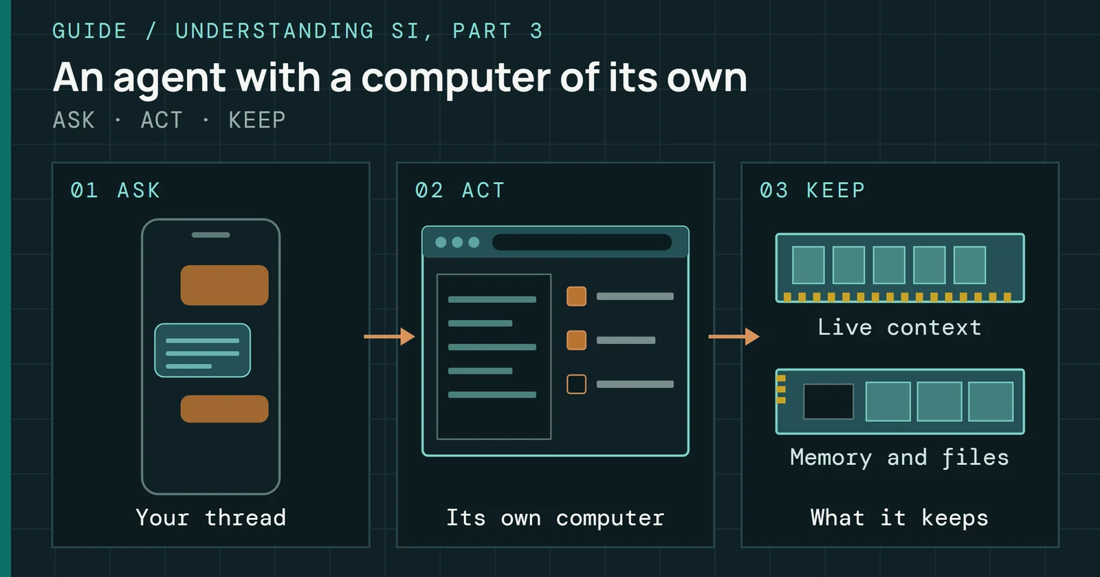
A language model does not look facts up. When ChatGPT, Claude, or Gemini answers, the model underneath has no database and no copy of the web to search. An assistant can be handed a search tool, but the model itself has none. It has a fixed set of trained numbers called weights, and every reply comes from multiplying the question through them. Meta’s Llama 3 paper counts 405B of them in its largest model.

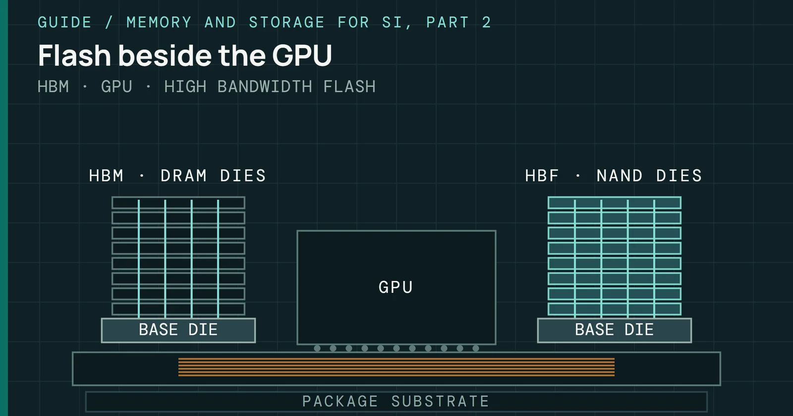
I come at this from storage, where the weights are data. For that model they come to about 810GB in a 16-bit format. They sit on an SSD, load into DRAM, and live in HBM beside the accelerator. A dense model reads all of them again for every word it writes. Where they sit in the memory and storage hierarchy decides how fast the answer comes.

Text goes in as numbers

Before a model sees anything, a tokenizer cuts the text into tokens, which are whole words, pieces of words, or punctuation. Each token is swapped for its position in a fixed list called the vocabulary. Llama 3 uses a vocabulary of 128K tokens, so every token becomes an ID between 0 and about 128,000. An ID works as an address. A model keeps an embedding table with one row per vocabulary entry, and the ID picks one row. Each row is a list of numbers called a vector. That row is all the rest of the model ever sees of the word. Its length is the model’s width, 16,384 numbers in Llama 3 405B.

128K rows × 16,384 numbers is about 2.1 billion numbers. At 2 bytes each, that is about 4.2GB of storage spent before a single layer has run.

Nobody fills those rows in by hand. Training sets them, and tokens that turn up in similar places in text end up with similar rows.

Weights: where the knowledge is kept

A weight is one number that an input gets multiplied by. Layers are mostly large grids of them, where each output sums the inputs after scaling each one by its weight. Every part of the model is stored this way, from the embedding table through the attention and feed-forward layers to the final layer that turns a vector back into token scores.

Counted up, they are the parameter number. Llama 3 405B has 405 billion trainable parameters across 126 layers. BF16 is a 16-bit number format, so each parameter takes 2 bytes. That makes 405 billion × 2 bytes = 810GB of weights. At BF16 the model does not fit in the GPU memory of one machine with eight NVIDIA H100 GPUs, so Meta served it across 16 GPUs on two machines.

No weight holds “Paris is the capital of France”. A fact the model states reliably is spread over many weights, and each weight takes part in many facts. Training keeps no list of sources either, so a model cannot say which document taught it something, and it can be wrong in the same confident tone it uses when it is right.

Attention reads the tokens before it

An embedding row carries no context, so “bank” starts as the same vector in “river bank” and in “bank account”. Attention is the core of the transformer introduced in the 2017 paper “Attention Is All You Need”, and it lets every token pull in information from the tokens before it.

Each token’s vector is multiplied by three weight matrices to make three new vectors called query, key, and value. For the current token, its query is compared with every earlier token’s key by a dot product. The result is one number that grows when the two vectors point the same way. A softmax turns those scores into shares that add up to one, and the token takes that mix of the earlier tokens’ values. In the paper’s notation it is Attention(Q, K, V) = softmax(QKᵀ / √dₖ) V, where Q, K, and V are the query, key, and value matrices and dₖ is the length of a key vector. When a model writes text, a mask keeps each token from reading anything that comes after it.

Llama 3 405B runs 128 attention heads side by side in each layer and stacks 126 layers, so a token’s vector is rewritten over and over by what it reads. Each layer also has a feed-forward block made of weight matrices with a nonlinearity between them, and it works on every token separately.

Attention costs memory, and the cost grows with the conversation. Every new token needs the keys and values of all the tokens before it, so a running model keeps them instead of recomputing them. Pope and colleagues at Google call this store the key-value (KV) cache. Unlike the weights, it changes while the model answers.

One token per pass

After the last layer, the vector at the final position goes through one more weight matrix that scores every vocabulary entry. A softmax turns the scores into probabilities, which the transformer paper describes as converting the decoder output to next-token probabilities. That list is the model’s whole output for one step, and it gives each of the 128K tokens a probability of coming next.

A program then picks one token, either the most likely or a random draw weighted by the probabilities, appends it to the text, and runs the entire model again. Say an answer runs 200 tokens, which takes 200 full passes. Between passes nothing carries over except the text so far and its KV cache, and each pass starts from the same frozen weights.

A setting called temperature controls how random that draw is. Set low, it pushes the draw toward the single most likely token. When I set up Google’s Gemma on my PC that way, it got stuck writing the same table row over and over until I raised the temperature.

“It just predicts the next word” is accurate about the output. Putting a sharp probability on the token after “The capital of France is” still needs the computation to carry what a capital is, which country is meant, and which city goes with it. So I think “just” is the wrong word.

Nobody wrote the weights

Training starts from random numbers and has one task, which is to predict each next token of a stretch of real text. Whatever probability the model gave the token that actually came next is scored, and the error becomes a small change to every weight. Each change goes in whichever direction would have made that token more likely. Carrying those changes back through many layers is backpropagation, which Rumelhart, Hinton, and Williams set out in Nature in 1986. Repeat it over enough text and the weights settle into values that predict well.

For Llama 3 405B, enough meant 15.6T text tokens and 3.8 × 10²⁵ floating-point operations of pre-training. No step in that run says “store this fact”. A fact gets into the weights because text that mentions it is easier to predict with it than without it, and the same pressure teaches grammar, arithmetic patterns, code structure, and the habits of an argument.

Pre-training gives a model that continues text. Assistants are trained further. Llama 3’s post-training ran several rounds of fine-tuning on example instructions and answers and of tuning on human judgments of which answer is better, each changing the weights again. A finished assistant knows what was common and consistent in its training text up to the date that text was collected, and it knows rare facts poorly.

Where the weights live

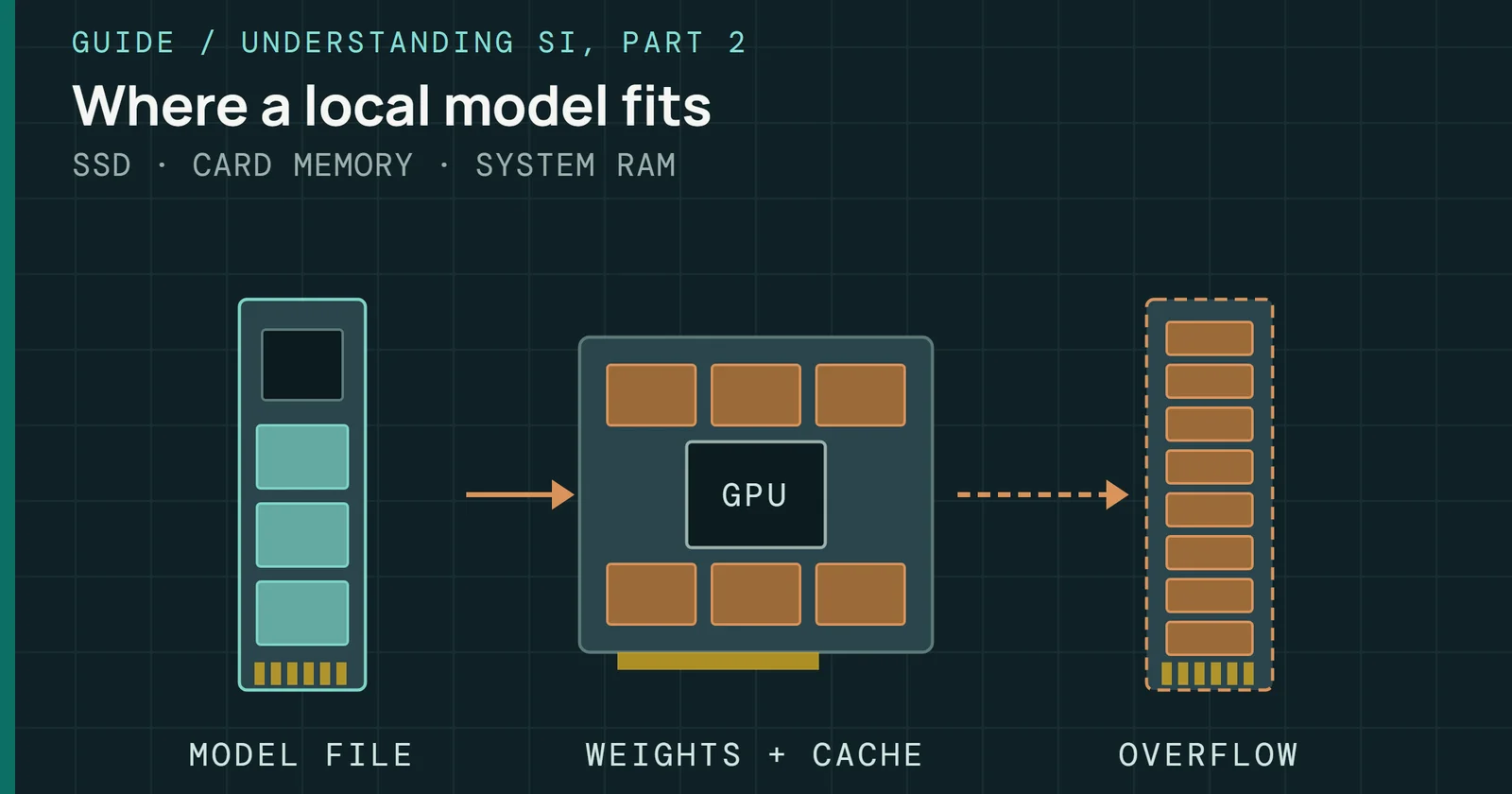
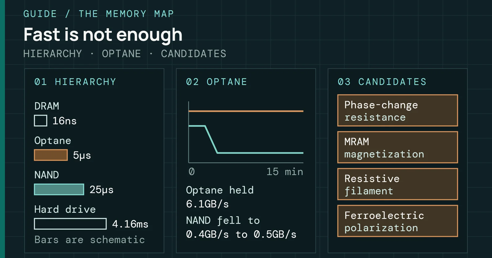
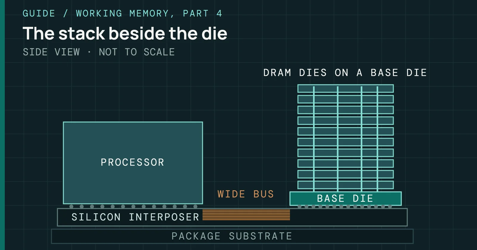
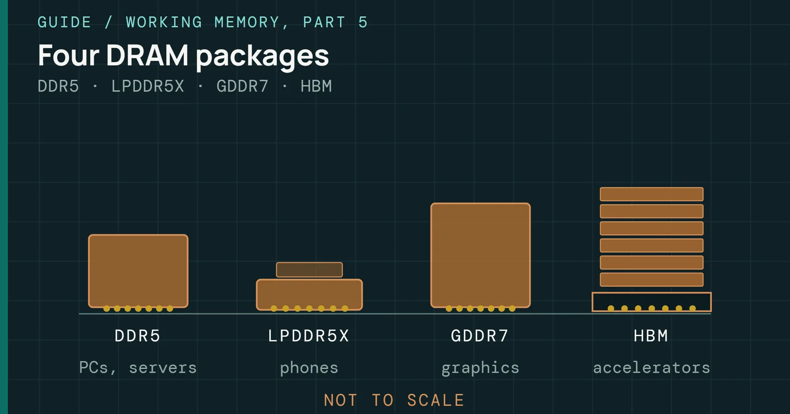
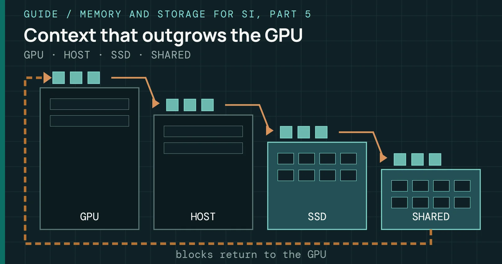
Weights are files. A served model sits on an SSD as a set of tensor files, is read into the host’s DRAM, and is copied into the HBM stacked beside each accelerator. Once the weights and the KV cache fit in HBM, nothing reads the SSD again while the model answers. The memory and storage hierarchy page gives the speed of each level on that path, and current memory ICs lists the HBM parts.

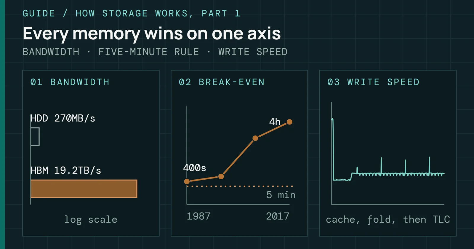
A dense model uses every weight for every token, so writing one token means reading every weight. Llama 3 405B is dense, so each token reads all 810GB. Google’s inference paper adds the KV cache to that load. Parameters and cache both move from HBM into the compute cores at every step, so a latency target is a memory bandwidth target.

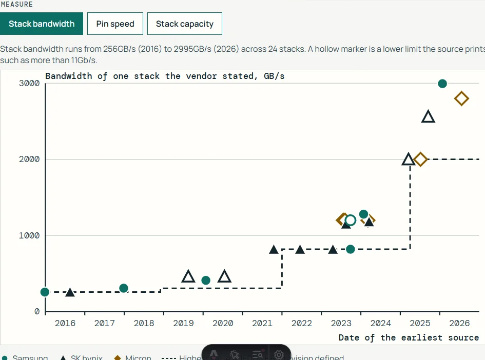
An NVIDIA H200 has 141GB of HBM3E at 4.8TB/s. Eight of them hold 8 × 141GB = 1,128GB, enough for the 810GB of weights plus a KV cache. Together they read at 8 × 4.8TB/s = 38.4TB/s. 810GB / 38.4TB/s is about 21ms per token. That is an estimated floor for one answer being written, before any compute time or traffic between GPUs. That works out to about 47 tokens a second at most, however fast the arithmetic units are.

Servers get more out of each read by working on many answers at once, since one pass over the weights serves every answer in the batch. A KV cache does not share that way, because each conversation has its own. In Pope’s example of a model over 500B parameters with standard multi-head attention, a batch of 512 at a context of 2,048 tokens needs a 3TB KV cache. That is three times the size of that model’s weights.

I see the same effect at desk scale. I run Google’s Gemma 4 26B locally through Ollama on my RTX 4090, which NVIDIA rates at 24GB of memory. In the Q4_K_M build Ollama serves, the model is a 17GB download. Ollama 0.33.3 reported 21.7GB in use on the card with a 64K-token context and 23.1GB with 128K, still entirely on the GPU. I took one reading at each size. Both runs used the same weights, so the extra 1.4GB is the price of the longer context. At 256K the model didn’t fit anymore, spilled into system memory, and the whole PC lagged.

My advice is to read an accelerator’s spec sheet from the memory lines up. For serving a model this size, HBM capacity and bandwidth say more than the compute figure. Bandwidth sets the 21ms floor for one answer. Capacity sets how large a batch’s KV caches can grow beside the weights.

Inside the model: what tracing has found

“Spread over many weights” leaves out what researchers can now see. With tools that are slow and cover small pieces of a model, they can find where some knowledge sits and watch some of it in use.

Facts in the feed-forward layers

Feed-forward blocks hold two-thirds of a transformer’s parameters, and a study led by Mor Geva shows they behave like key-value memories. Each key responds to a pattern in the input text, and its value pushes the output toward the tokens that tend to follow that pattern, with shallow patterns in the lower layers and patterns of meaning higher up.

Meng and colleagues’ ROME paper (Rank-One Model Editing) went further with OpenAI’s GPT-2 XL. They gave the model a factual prompt, added noise to the subject’s words, and restored one internal state at a time to see which one brought the right answer back. Feed-forward blocks in the middle layers, at the last token of the subject’s name, were decisive. Changing the weights of one of those layers by a small, targeted amount made the model state that the Space Needle is in Paris.

Traced steps inside Claude

In 2025 Anthropic traced how Claude 3.5 Haiku works through short prompts, mapping which internal features feed which. The full paper, “On the Biology of a Large Language Model”, has the case studies, and four of them bear directly on how a model knows things.

• Asked for the capital of the state that contains Dallas, the model activates a feature for “Dallas is in Texas”, then one for “the capital of Texas is Austin”. When the researchers swapped the Texas features for California ones, the answer changed to Sacramento.
• Writing a rhyming couplet, the model picks the rhyme word before it writes the line. With “rabbit” planned and then removed, it wrote a line ending in “habit” instead.
• For 36 + 59, one path estimates the rough size of the sum while another works out the last digit, and the two combine to give 95. Asked how it added, the model describes carrying the 1, though it did not use that method.
• Declining is the default. A circuit that says “not enough information” stays on unless a “known entity” feature switches it off. When a name is familiar but the facts behind it are not, that switch can fire wrongly, and the model makes something up.

Anthropic is plain about the limits. Even on short prompts the method captures only a fraction of the computation, and understanding the circuits for a prompt of tens of words takes a few hours of human work.

Why written steps help

A model gets one pass per token, and a pass has a fixed number of layers. That suggests why writing steps out helps. Steps that one pass can’t hold in sequence can be spread across many passes. Each written token is read back through attention on the next pass, so the text and its KV cache work as scratch memory, and each of those tokens costs a full pass. When I first ran Gemma with its thinking mode on, it spent its whole output budget thinking and never wrote the answer I’d asked for, so I run it with thinking off.

A Google study led by Jason Wei tested chain-of-thought prompting. That puts worked examples with their steps written out into the prompt. The study found that it improved arithmetic, commonsense, and symbolic reasoning. With eight such examples, Google’s PaLM 540B set the best result at the time on GSM8K, a set of math word problems.

At the 2025 International Mathematical Olympiad (IMO), the competition’s own coordinators scored an SI result. Google DeepMind reports that an advanced version of Gemini Deep Think solved five of the six problems in full for 35 of 42 points, working in natural language within the 4.5-hour limit. IMO coordinators judged that score gold-medal standard, and DeepMind was in the first group of labs to get that verdict. DeepMind also says it trained this version with new reinforcement learning methods and gave it a curated set of solved problems and hints. DeepMind adds that the coordinators’ review didn’t extend to validating the system behind the answers.

Written reasoning can differ from the computation behind it. On a hard calculation, Anthropic’s tracing found no sign of the steps Claude wrote out as its working.

What to watch

Tracing has to scale before anyone can check where a fact sits outside small cases like the Space Needle edit. At hours of human work for a prompt of tens of words, I don’t expect to see tracing follow a model the size of Llama 3 405B through a real conversation soon.

Then there’s grading. An OpenAI paper led by Adam Tauman Kalai argues that wrong answers come from the same training that produces right ones, because a model is rewarded for guessing instead of saying it is unsure. It ties a lower bound on the error rate to how many facts appear only once in the training data. Claude’s default-decline circuit fits that reading. If the paper’s right, I’d watch how models are graded well ahead of how large they get.

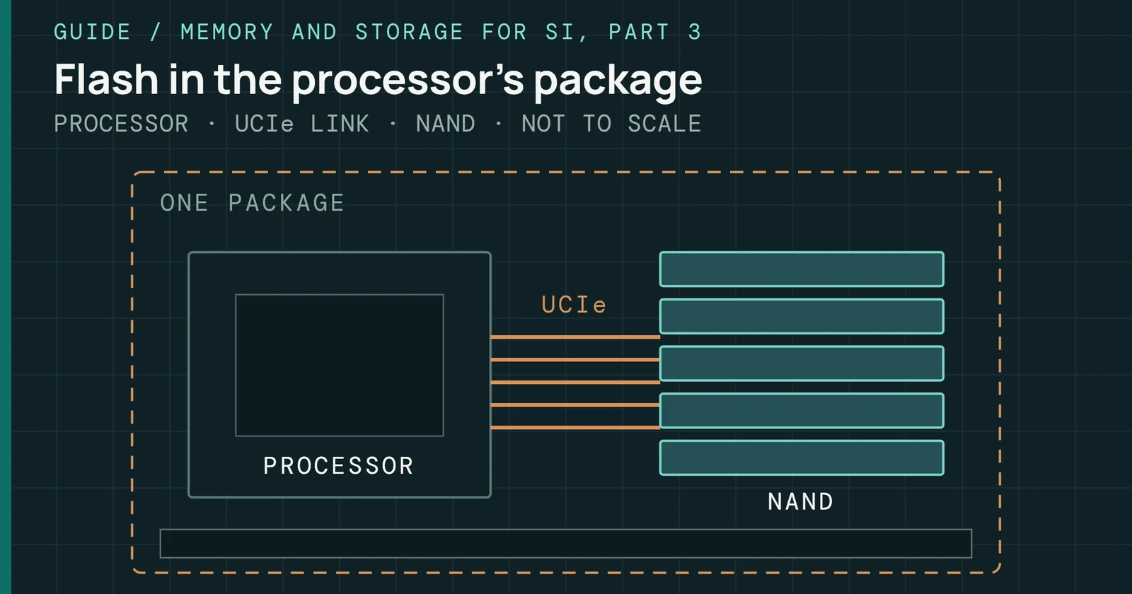
On the hardware side, Memory and Storage for SI, Part 2: High Bandwidth Flash looks at flash as a memory tier beside the accelerator, a place for weights and KV caches besides HBM. If that works, flash would be read while a model answers, and not only when it loads.