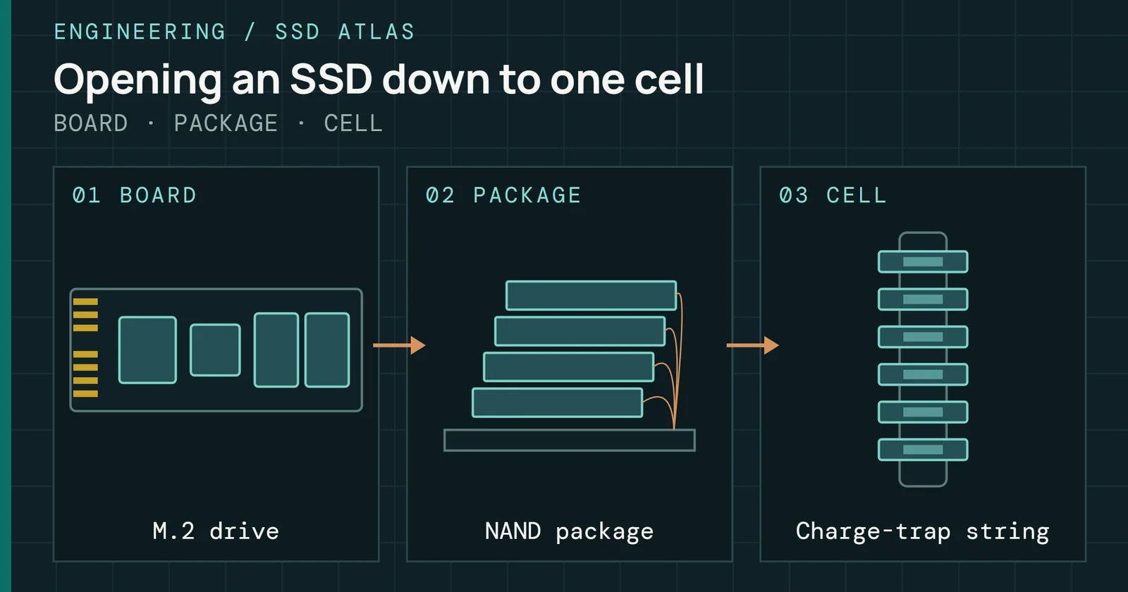
A cell is a transistor that holds charge, and it becomes storage only when trillions of them are organized into structures you can address, read, write, and erase. Each level of that hierarchy shares something among its cells. A string shares contacts, a wordline shares a control gate, a block shares erase bias, and planes and dies share a data path.
Flash Foundations
Flash Foundations, Part 3: From Cell to Die
Follow cells into pages, blocks, and dies to understand how NAND is organized.
On this page 16 sections
Part 2 covered the cell, including trapped charge, threshold voltage (Vt)Threshold voltage, Vt, is the gate voltage at which a flash cell starts to conduct. The stored charge shifts it, and the controller reads data from it., and why density costs endurance. This part scales that cell into strings, wordlines, pages, blocks, planes, dies, and packages, which are the units that firmware and the controller actually address.
Why can a drive write a page but only erase a blockFlash programs one page at a time but erases a whole block at a time, which is why changing a small amount of data causes much more internal work.? Why does a read disturb cells it never asked about, and why do the pages on one wordlineA wordline is the conductor that crosses a row of cells and sets the gate voltage for every cell on it. One wordline holds one or more pages. age at different rates? By the end of this part you can trace one operation from a cell to a die and answer both, along with why erasing forces garbage collection (GC)Garbage collection copies the valid pages out of mostly stale blocks and erases those blocks, so there is always free space for new writes. and why a larger drive on the same controller often wins. Skip the hierarchy and GC looks like a firmware quirk, write slowdowns look random, and two errors with the same NVMe status code look like one failure even when the silicon behind them differs.
NOR versus NAND: why cells share contacts
A cell that stores one to four bits is useless alone. You need cells in structures you can address cheaply. The series string is why NAND exists as a product, because it cuts contacts and interconnects per cell. Every extra contact costs area, yield, and reliability. Wire cells in series and the die gets dense and cheap.
NORNOR flash wires cells in parallel for fast random reads of single bytes. NAND wires them in series for much higher density at the cost of page-wise access. came first. Masuoka’s 1984 flash cell used one transistor per bit and three layers of polysilicon, with the third working as an erase gate, and it programmed by hot-carrier injection like an EPROM. A NOR array gives every cell its own contact to a bitlineA bitline is the wire that runs across many strings and carries the sensed signal to the page buffer. Cells on one wordline share it in turn., so any single cell can be read directly at random-access speed. Code can therefore run straight out of NOR. The price is area, since a contact per cell puts it near 10F², where F is the minimum feature size.
Masuoka’s 1987 NAND structure put cells in series and shared the contacts. That paper reports a 6.43µm² cell at a 1.0µm design rule, 30% less area per bit than a conventional EPROM cell at the same rule. Micron’s TN-29-19 NAND primer puts NAND at about 4F² against 10F² for NOR.
NOR versus NAND: why cells share contacts
NOR gives each cell a contact; NAND shares one across the string
Fewer contacts per cell is the density gain; a slower first read is the cost
Figure 3.1 puts the two wirings side by side. Three NOR cells need three contacts, while four NAND cells share one, which is where the density gap comes from.
A series path has a cost of its own, because a NAND stringA NAND string is a column of cells connected in series between a bitline and the source line, with a select transistor at each end. passes only about 100 to 200nA, and the read threshold sits at tens of nA, so sensing is slower. The TN-29-19 note puts NAND random access at 25µs for the first byte against 0.075µs for NOR, so NAND traded fast random reads for density. Beyond NAND puts both on the same memory ladder as DRAM, Optane and the memories that still hope to join them.
NOR versus NAND: why cells share contacts
Cells form strings, strings share wordlines, and pages fill a block
Series wiring makes NAND dense; shared gates make the page the write unit
Figure 3.2 stacks the levels this part covers, from the cell up to the die, and the sections below follow it in order. Series wiring has a second cost, shared bias. An operation on one cell drives every cell in its string, and a wordline drives every string in the block. Shared bias is the physical root of read disturbRead disturb is the slow charge gain in unselected cells caused by the pass voltage applied to them every time a neighboring page is read. and program disturbProgram disturb is unwanted charge added to cells that should stay unchanged. Self-boosting raises the channel voltage of inhibited strings to reduce it..
Cells and strings: the series connection
NAND cells sit in series. One Toshiba NAND patent describes strings of four, eight or sixteen cells, with eight as the worked case. A drain selectThe drain and source select gates connect a string to its bitline and to the source line, so only the chosen strings take part in an operation. transistor caps the top of the string and a source select transistor the bottom.
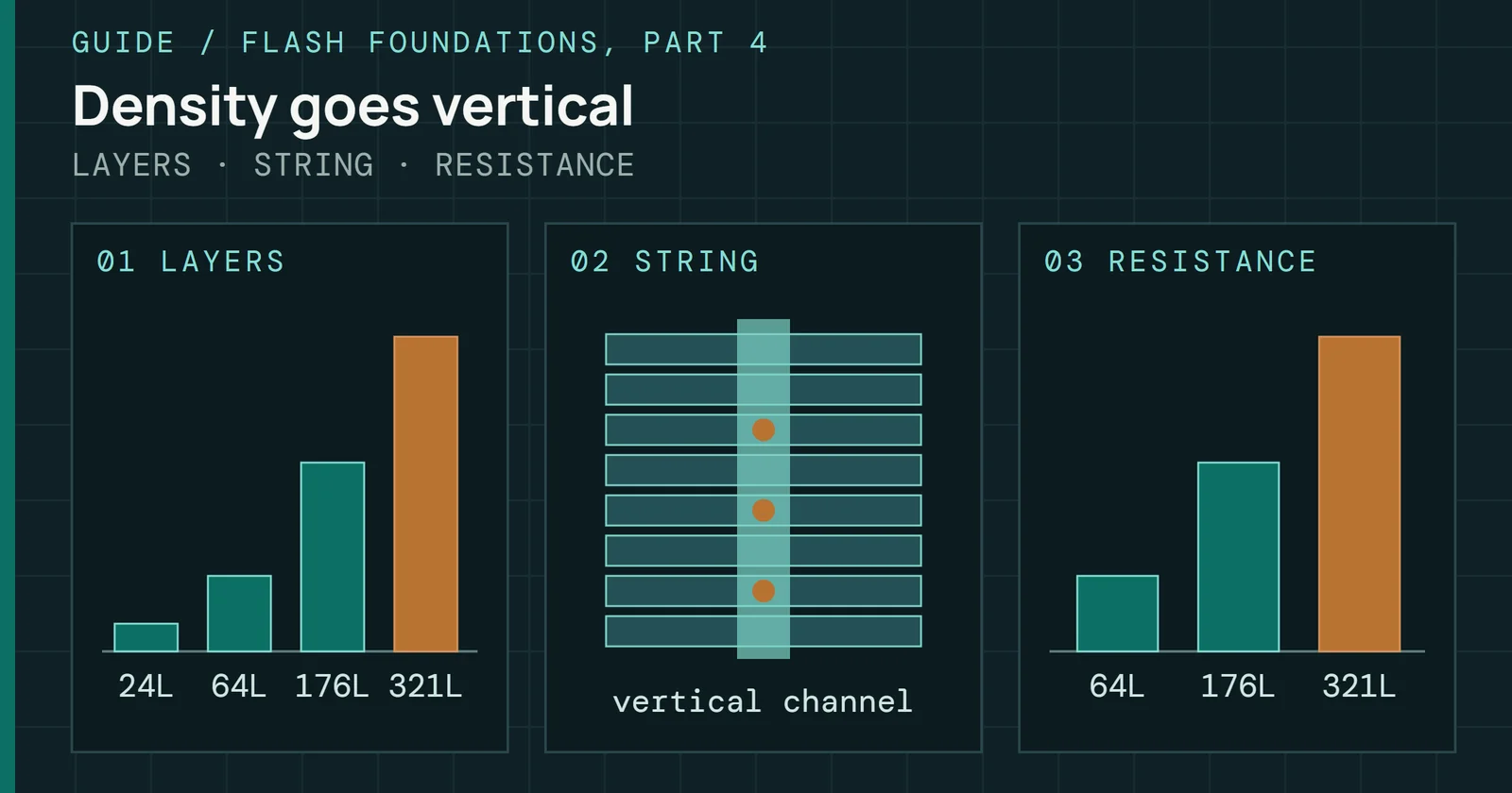
Planar strings grew with the nodes. One 0.13µm 1Gb part raised its string from 16 to 32 cells, and strings of 64 and 128 cells followed. Early 3D strings started at 24 wordline layers and ran to 64, and mid generations moved to 96 to 128. As of October 2026, high-layer 3D NAND stacks run 218 to 321 layers, and SK hynix’s 321-layer part has 321 active wordlines.
To read one cell, every other cell in the string has to conduct, regardless of what it stores. Current runs drain to source. The cell you asked about is the one that can interrupt that path.
Cells and strings: the series connection
A read turns on every cell in the string except the one it asks about
One string, one selected wordline
Figure 3.3 shows one string under read. The selected wordline gets the read voltage, every other wordline gets a pass voltagePass voltage, Vpass, is applied to every unselected wordline during a read so those cells conduct whatever they hold and the selected cell decides the current. high enough to turn its cell on, and the sense circuitA sense amplifier compares the current or voltage of a selected cell against a reference to decide which stored level the cell holds. watches whether current reaches the source line.
The consequence is read disturb. Every read stresses the cells on every unselected wordline in the block, not just the target string. Tens of thousands of reads or more on the same block, depending on generation and wear, shift Vt in cells you never meant to touch. Firmware keeps a read count per block and refreshes it before that accumulated stress becomes an uncorrectable error, one that error-correcting code (ECC)Error-correcting codes add parity bits to each block of data so the controller can find and fix bit errors on read. can no longer fix.
How a read works
The read itself is a race. Series resistance limits the current a string passes, so a longer string passes less and takes longer to sense. That current is tiny, and no circuit measures it directly. The page bufferThe page buffer is a set of latches on the die that hold one page of data on its way to or from the cells. integrates it onto a capacitor in three steps. First it charges each selected bitline, by about 1V in a published example that takes 10µs. A bitline is long and carries a lot of capacitance, so this precharge is a large share of the read time. Next the selected wordline gets the read voltage, the other wordlines get the pass voltage, and the bitline is released to discharge through the string. Last, after a fixed window, a latch compares the bitline voltage with a trip level and stores a 1 or a 0.
How a read works
A read charges the bitline, then times how fast the cell drains it
Bitline voltage over one read, 2pF bitline
Figure 3.4 shows the bitline of a conducting cell sagging during evaluation while the bitline of a blocking cell holds its charge. The latch flips only if the voltage has fallen to the trip level when the window closes. Charge integration sets the rest. The voltage change is ΔV = I × T / C, so the current a cell must exceed to read as conducting is I = ΔV × C / T, with ΔV the swing the latch needs, C the bitline capacitance and T the evaluation window. Published sensing studies of sub-30nm parts put the bitline at about 2pF at best, treat a swing below about 100mV as impractical and run the window near 10µs in practice. That makes the threshold 100mV × 2pF / 10µs = 20nA. Lengthening the window lowers the threshold current, and shortening it raises it.
Each read level is therefore defined by both a current and a time, and the wordline voltage alone does not fix it. Every extra read level repeats the evaluate and latch steps, which is why a page that crosses more references takes longer to read. Page types counts the levels each page needs.
Sensing schemes differ in how they handle the bitline. Neighboring bitlines couple capacitively, so early NAND read every other bitline and grounded the rest as shields. Tanaka and colleagues report that a shielded bitline cut bitline-to-bitline noise in their 0.7µm part from 700mV to 35mV, with a 2.5µs random access time. Shielded designs typically read a wordline in two passes, even bitlines then odd. The all-bitline (ABL) scheme holds every bitline at a constant voltage and senses current instead, so no neighbor swings and a whole wordline reads at once. Cernea and colleagues introduced ABL with current sensing in a 16Gb four-state multi-level cell (MLC) part at 56nm.
The erased state sits at a negative Vt, and a read has to tell it from the first programmed state. Rather than drive the wordline negative, designs can raise the source line, which has the same effect as lowering the gate. Shibata and colleagues report a source-bias negative sense in a 1.33Tb quad-level cell (QLC) part.
Program disturb and self-boosting
Programming has its own way of protecting the strings you did not choose. The other strings on the wordline get their channels left floating and the shared wordlines rise, so the channel rises with them. Engineers call that self-boosting. It cuts the field across their cells, but the same pass voltage stresses the cells on unselected wordlines of the string being programmed, so the pass voltage has to sit between two stresses.
Program disturb and self-boosting
A floating, boosted channel keeps a skipped string from programming
Two strings that share one wordline
Figure 3.5 puts two strings that share a wordline side by side. In the programmed string the channel is held low, so the cell on the highlighted wordline sees a strong field and takes charge. Meanwhile the inhibited string’s channel floats and boosts, which cuts the voltage across the tunnel oxide, so that cell keeps its Vt.
Program a wordline and the high voltage also hits cells you did not select. Inhibited cells on that wordline in other strings see the program voltage minus their boosted channel voltage, which is why self-boosting works, and cells on the other wordlines see the pass voltage. Planar NAND coupling grew as each node shrank the lateral gap. 3D NAND separates its stacked wordlines with interlayer oxide. As makers thin those layers to fit more of them in, wordline pitch shrinks and coupling climbs again. Firmware answers with write order. Under the program-order rule, firmware programs wordlines sequentially through the stack instead of at random, so the same neighbor does not eat repeated coupling. Part 4 returns to write ordering in tall stacks, and Part 5 covers the multi-pass program sequence rules.
Three more positions take stress. A cell on an unselected wordline in the string being programmed sees only the pass voltage. A cell on an unselected wordline in an inhibited string is mostly shielded by the boost. The edge cell beside the select gate is the exception, because gate-induced drain leakage (GIDL)Gate-induced drain leakage erase raises the channel voltage at the end of a string until holes are generated that erase the cells above. there makes hot electrons that inject into wordline 0. Part 4 covers that edge disturb and the dummy wordlines that shield it.
The pass voltage has a window with two walls. If it sits too low the channel boosts too little, so inhibited cells program by mistake. Too high and the programmed string takes pass disturb. Planar designs raised the boost ratio with a channel boost capacitance structure, and Park and colleagues report that a dynamic pass voltage scheme cut program failures by over 40% after 30,000 program/erase (P/E) cycles and about doubled the pass voltage window margin on a 42nm MLC test chip (JSSC 2010).
Write order has two physical reasons. Coupling comes first. Lee and colleagues measured about a 0.2V shift from neighbor coupling in multilevel operation at a 0.12µm design rule, and a fixed order limits how many neighbors change after a cell has been verified.
Background pattern dependency is the second reason. A string’s current depends on the Vt of every other cell in it, so a cell’s read Vt can shift with what its neighbors later hold. Designs typically fix the program orderPages in a block must be programmed in a set order, usually from the first wordline to the last, to limit disturb between neighboring cells. so that shift is predictable instead of random.
Both errors come from operations that were never supposed to change those cells. Trigger, target, and accumulation pattern are different, and so is the firmware defense.
| Mechanism | Physical trigger | Cells at risk | Accumulation rate | Firmware defense |
|---|---|---|---|---|
| Read disturb | A pass voltage on all unselected wordlines in the block during every read | Cells on every unselected wordline in the block, across all strings that share those wordlines | Proportional to the block’s read count, builds over tens of thousands of reads or more | Per-block read counter, data relocation before the threshold is reached |
| Program disturb | A high, stepped program voltage on the selected wordline, plus a pass voltage on the others | Inhibited cells on the selected wordline, plus cells on unselected wordlines in the same block | Grows with program operations across the block, and accelerates in tall stacks with tighter spacing | Fixed sequential wordline write order, voltage shaping between wordlines, ECC headroom |
Neither error is fixed in place. Firmware keeps count, watches and relocates before ECC runs out, and Part 7 covers how that refresh is managed.
Wordlines and pages
Cells in the same position across strings share a control gate. That horizontal run is the wordline. Activate it and the cells on it in the selected string group can be read or programmed together. Cells on one wordline hold one page for each stored bit. A page is the smallest unit you can read or write. In modern 3D NAND that is typically around 16KB, plus spare bytes.
Wordlines and pages
One page is the cells along one wordline, not several data chunks
A block face with five strings and four wordlines
Figure 3.6 corrects a common picture. One page is a single run of cells along one wordline, which means a wordline holds no stack of separate 16KB chunks. A triple-level cell (TLC) wordline carries three such pages, each for one stored bit, as the next section shows. Spare cells at the end belong to the same page. Read the page and the die returns the user data and the spare area together.
Before data hits the cells, it gets scrambled. Many SSD controllers XOR the data with a pseudo-random key before it reaches the NAND. That key is usually seeded from the data’s logical address, and the controller applies the same key on read to undo it. Electrical effects are the reason. Constant data skews state occupancy and shifts read levels through pattern-dependent string current, and repeated patterns can line up worst-case cell-to-cell interference. Scrambling makes even compressible or constant data look mixed enough to sense and retain. The host never sees the scrambling, and NVMe logs do not mention it. A raw NAND dump that skips descrambling looks corrupted even when the cells are fine.
Some dies also adjust their own read levels from stored counts, and Part 8 covers read retry.
Each page also has an out-of-band (OOB)The spare, or out-of-band, area is extra bytes on every page that hold error-correction parity and controller metadata. region the host cannot address. Older generations used 64 bytes per 2KB page, as Micron’s TN-29-19 shows. Modern 16KB-page 3D NAND carries around 2KB of spare per page for larger error correction. OOB commonly holds low-density parity-check (LDPC)LDPC is a code whose decoder passes confidence messages back and forth until the errors resolve. It corrects more errors than BCH, especially with soft input. parity, block metadata, bad-block marks, and often a reverse-mapping entry that holds the logical page number. NVMe does not expose it as capacity. Part 6 shows how firmware uses that per-page metadata to find which writes finished after a dirty shutdown. In raw analysis, missing or inconsistent OOB on a page that should have data usually means a program that died mid-write, or damage beyond what ECC already reported to the host.
Page types: how 1-2-4 coding splits one cell into three pages
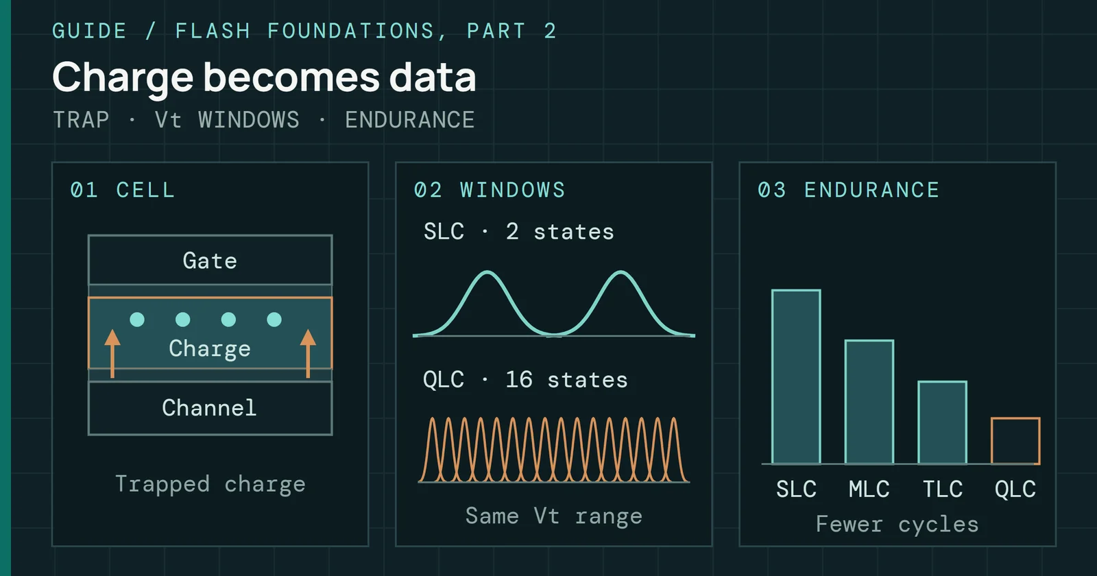
A cell stores more than one bit by holding one of several threshold voltages. A single-level cell (SLC)A cell storing n bits needs 2 to the power n voltage levels: two for SLC, four for MLC, eight for TLC and sixteen for QLC. stores one bit in two states. A TLC stores three bits in eight states, and a quad-level cell (QLC) stores four bits in sixteen. Those bits belong to different pages. In a TLC, each cell gives one bit to each of the lower page (LP), middle page (MP), and upper page (UP)In a multi-bit cell each bit belongs to a different page type: lower, middle, upper and, for QLC, extra. Each type needs a different number of reads. of its wordline, and a QLC cell adds an extra page (XP).
Which bit goes to which page is set by a code. Adjacent states get bit patterns that differ in exactly one bit, which is a Gray code, so a cell that drifts into the next state causes one bit error instead of several. 1-2-4 codingA 1-2-4 coding assigns bits to voltage levels so the lower page needs one read reference, the middle two, the upper four. Gray code keeps neighbors one bit apart. is a common way to spread that code across pages, and the lower page flips at one boundary between states, the middle page at two, and the upper page at four. A published survey’s TLC mapping reads the lower page with one reference voltage, the middle page with two and the upper page with four.
Page types: how 1-2-4 coding splits one cell into three pages
The same eight states give the three pages one, two and four reads
One Gray-code assignment for a triple-level cell; vendors differ
Figure 3.7 marks with dots the read references each page must use. A page error needs a cell to cross one of that page’s references. Lower-page bits change only at R4, so that page has one reference to cross and needs one read level. Upper-page bits change at R1, R3, R5, and R7, so that page has four to cross and needs four read levels. Under equal drift, the upper page collects more errors, and it takes longer to sense. This is one assignment. Vendors use others, and the counts differ by scheme. A 144-layer QLC paper names 1-2-4-8 as a QLC code and uses 1-2-6-6 instead, which cut its maximum read time by 25%.
Those counts follow from the code. A cell with n bits has 2ⁿ states and 2ⁿ − 1 boundaries between them, and the code spreads those boundaries across n pages. Averaged over pages, a read takes (2ⁿ − 1) / n senses: 1 for SLC, 1.5 for two bits, about 2.3 for TLC and 3.75 for QLC. Program verifyProgram-verify alternates a program pulse with a read check. Cells that reached their target stop receiving pulses, and the rest continue. can need up to 2ⁿ − 1 levels per pulse too. Multi-level parts use multi-pass programming to suppress neighbor coupling, and Part 5 covers the sequences.
Page types differ in more than read levels. The coding and the program order give each one a different profile.
| Page (multi-pass view) | Programming order | Read levels (1-2-4 style) | Relative error rate |
|---|---|---|---|
| Lower page (LP) | First | 1 | Lowest |
| Middle page (MP) | Second | 2 | Medium |
| Upper page (UP) | Third, last in TLC | 4 | Highest in TLC |
| Extra page (XP), QLC only | Fourth, last in QLC | 8 in a 1-2-4-8 style code | Highest in QLC |
In multi-pass schemes, upper pages program last, into the full eight-level TLC or sixteen-level QLC distribution. In one-shot schemes the pages of a wordline go in together, but the upper page still has the most read references, so it has the most boundaries where disturb and retention can push a cell across. On TLC at moderate program/erase (P/E) cyclesA program/erase cycle is one write of a block followed by its erase. Each cycle wears the oxide, and the cell type sets how many cycles it tolerates., upper-page raw bit error rate (RBER)Raw bit error rate is the fraction of bits read from the NAND that are wrong before error correction is applied. is usually higher than lower-page RBER on the same block, by an amount that depends on the coding scheme, generation, and wear, and firmware has to budget for that gap.
Some firmware keeps critical metadata in SLC-modeSLC mode, or pseudo-SLC, runs a multi-level block as one bit per cell. It writes faster and survives more cycles, but holds a fraction of the data. blocks, which are programmed one bit per cell, or on lower pages, and lets user data take the upper-page error rate. Firmware that ignores page type has to size ECC for the weakest pages everywhere.
Blocks: the erase unit and the root of GC
The series connection also draws the erase boundary. A string lives in a block, and the block is the smallest thing you can erase. You can write a page. You cannot overwrite it, because programming only adds charge and removing it takes an eraseFlash cannot overwrite a page in place. The cells must first be erased to the lowest level, and erase works only on a whole block. bias that the whole block shares. Erase resets every cell in every page at once. A block holds 1,024 or 1,536 pages in Micron’s 2016 3D parts and 2,304 in Frontgrade’s, which is tens of megabytes depending on page sizeA page is the smallest unit a NAND die programs or reads, commonly 16KiB of data plus a spare area for error-correction codes and metadata. and generation.
Everything above NAND lives with this constraint. The write unit is a page, around 16KB, and the erase unitA block is the smallest unit that can be erased. It holds hundreds to thousands of pages, so one erase clears megabytes of data at once. is a block, tens of megabytes.
Blocks: the erase unit and the root of GC
A 4KB update writes a new page and later erases a whole block
The write unit is a page, the erase unit is a block
The figure sets the two units side by side. A 4KB update does not erase 4KB. It is written to a fresh page alongside other pending writes and marks the old 4KB copy invalid, and the stale copies pile up inside their blocks.
Sequential work fills blocks and moves on. Random small writes scatter invalid pages across many blocks, so each GC cycle touches more of them. GC copies the still-valid pages out and then erases the block, and every copy is a write the host never asked for. The ratio of NAND bytes written to host bytes written is the write amplification factor (WAF)Write amplification factor is the data written to NAND divided by the data the host wrote. A value of 1 means no extra internal writes.. Part 7 covers how firmware picks victims, separates hot and cold data, and levels wear, and it defines WAF.
Planes give parallelism within a die
A die is split into planes. Tom’s Hardware’s 2021 review of the Samsung 980 reports two planes per die, and Micron’s 232-layer die, announced in July 2022, has six. Each plane has its own page buffer. Multi-plane commands usually run planes in lockstep, and some newer parts can also read each plane independently. A multi-plane operation lets the controller work on more than one page in the same die at once. That means more throughput from the same die count.
Planes give parallelism within a die
One command can work on the same page in every plane at once
One die with four planes, each with its own page buffer
Figure 3.9 shows why planesA plane is an independent set of blocks on a die with its own page buffer. A multi-plane operation runs the same command on several planes at once. help. Each plane has its own page buffer, so the array operations overlap, while the die’s single I/O path is shared.
Two-page read timing shows the gain. Let tR be the array sense time and tOUT the time to move one page over the channel. Reading two pages one after the other costs 2 × tR + 2 × tOUT. Multi-plane reads sense both pages at once and pay tR + 2 × tOUT, because only the transfers take turns. Cache reads sense the second page while the first one moves out, so they cost tR + tOUT + the larger of tR and tOUT. When tOUT is the larger, that equals the multi-plane time. When tR is the larger, sensing stays the bottleneck and multi-plane wins.
| Read mode, two pages | Time | Datasheet example (µs) |
|---|---|---|
| One page after the other | 2 × tR + 2 × tOUT | 203.7 |
| Multi-plane | tR + 2 × tOUT | 143.7 |
| Cache | tR + tOUT + max(tR, tOUT) | 175.9 |
The example uses one real part, the 4Tb TLC NAND part in Frontgrade’s datasheet. It lists a typical single-plane page read of 74µs, a typical multi-plane read of 88µs and NV-DDR3 at 667MT/s, which is 667MB/s on its eight-bit bus. A full page with its spare area is 18,592 bytes, so tOUT is 18,592B / 667MB/s, about 27.9µs. The multi-plane row uses the 88µs multi-plane time in place of tR. Here tR is larger than tOUT, so sensing is the bottleneck and multi-plane finishes first.
Many parts need the same page address in each plane for one multi-plane command, though later ONFI revisions, starting with 4.2 in 2020, relaxed some of those restrictions. On such a part, page 47 in plane 0 and page 312 in plane 1 cannot go in one command. Firmware has to know which blocks share a compatible address, which is why the flash translation layer (FTL)The flash translation layer is the firmware that maps host addresses to physical flash locations and hides the rules of erase blocks and wear. groups blocks across planes and dies into superblocks and treats each as one unit. Writes stripe, and erases clear the members together. Part 6 covers how. Without that grouping, even fast NAND is stuck at single-plane, single-die speed.
Wear breaks the pairing, and a block can retire while its partner in the next plane is still healthy. Part 6 covers how firmware remaps it, and what that costs the stripe.
Copy-back is a GC shortcut on the same die. It reads a page and programs it to a new location without dragging data through the controller, which keeps the channel free. It only works inside the die, usually the same plane, and it skips the ECC path that would clean errors before rewrite. Use it only on low-RBER pages. Copy a dirty page and you plant those errors in the destination.
Dies, packages, and the full parallelism stack
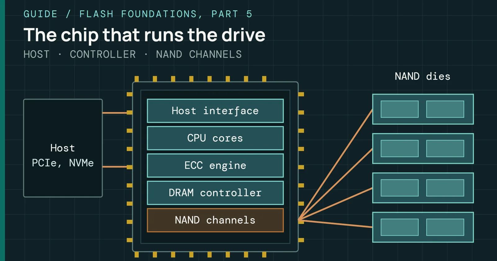
A die is the full array on one piece of silicon, holding cells, strings, wordlines, blocks, and planes. A packageSeveral dies can share one package, stacked and connected by wire bonds or through-silicon vias, which adds capacity without more board area. holds one or more dies, and a drive carries several packages. The controller talks to dies over channels, parallel paths that let more than one die work at once. Silicon Motion’s SM2262EN brief lists eight NAND channels and four chip enables per channel. With one die behind each chip enable, 32 dies can work in parallel, and each die has two to six planes. Channels × dies × planes is the theoretical ceiling.
Dies, packages, and the full parallelism stack
Capacity often buys parallelism, not faster silicon
Same controller, same NAND: more dies at the larger capacity
Each level of the stackFlash gets its speed by working in parallel at several levels: channels carry data, each channel serves several dies, and each die has several planes. multiplies the one below it, so the ceiling is the product of all three. Capacity and performance therefore travel together at a given tier. A 2TB drive on the same controller and NAND as a 500GB drive has more dies, more planes, and often more live channels. With 512Gb dies that is about 32 dies against 8. The ceiling is higher because there are more execution units rather than faster silicon. A spec sheet may list the same peak sequential read number across capacities. As of October 2026, the SN850X datasheet does so for its 1TB, 2TB, and 4TB models. Sustained mixed-load throughput usually does not match. In the Parallelism Lab, pick a die and a controller, then raise the capacity and watch which limit sets the write speed.
Each level has one job and one constraint that the levels above it inherit:
| Level | Function | Typical scale | Key constraint |
|---|---|---|---|
| Cell | Stores charge | 1 to 4 bits | Analog, wears with cycling |
| String | Series connection | 8 to 321 cells, by generation | Read disturb |
| Wordline | Parallel read and write | Spans all strings | Shared activation |
| Page | Write unit | 16KB typical | Cannot overwrite in place |
| Block | Erase unit | Tens of MB | Must erase the entire block |
| Plane | Parallelism within a die | 2 to 6 per die | Positional coordination |
| Die | Complete array | Tens to hundreds of GB | Channel throughput |
| Package | Physical chip | Several dies | Thermal, power |
In CMOS-under-array (CuA) and periphery-under-cell (PUC)CMOS under array, called CuA or periphery under cell, places the control circuits beneath the memory array instead of beside it, saving die area. designs, peripheral logic sits under the array on the same die and reaches it through in-die vertical contacts instead of TSVs. Part 4 covers CuA, PUC, and bonded designs.
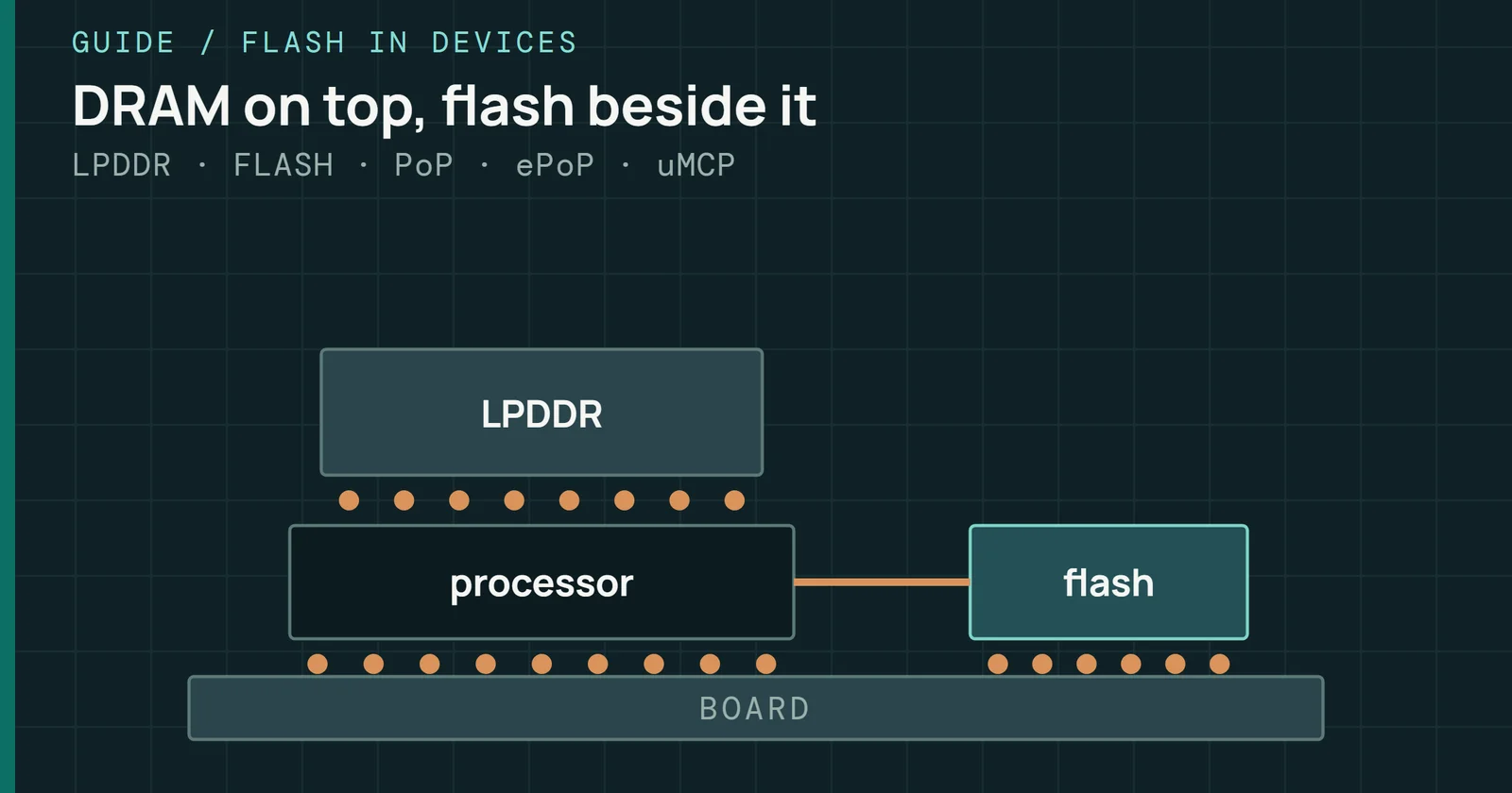
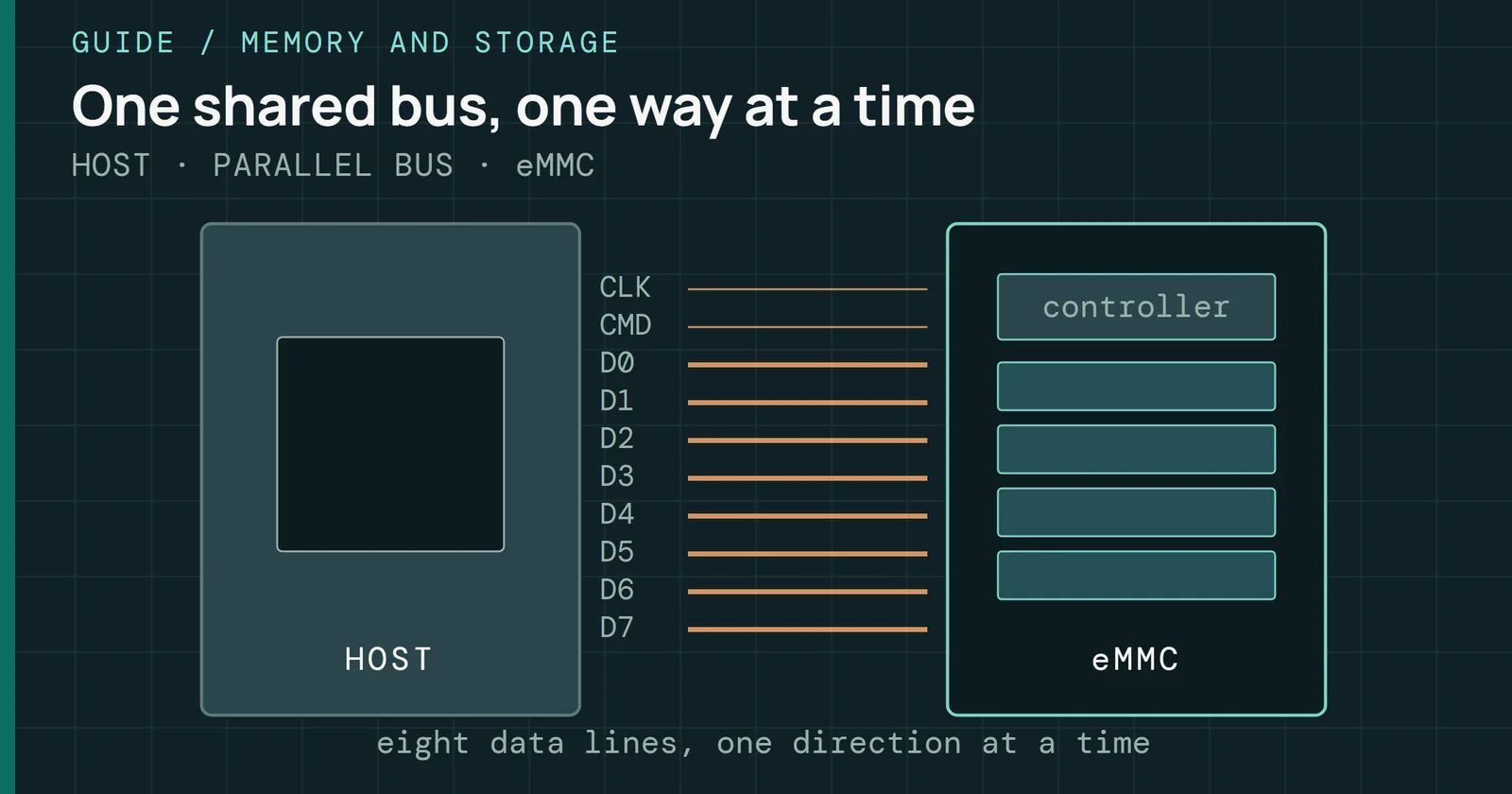
Capacity scales with dies per package and packages per board, which is why many high-capacity M.2 drives put NAND on both sides. In its 2021 review, Tom’s Hardware describes the Samsung 980 as using one NAND package holding up to sixteen 512Gb dies. At the small end, the controller and NAND can share one package. For example, Silicon Motion’s SM2263XT enables 11.5 × 13mm ball grid array (BGA) SSDs, and embedded MultiMediaCard (eMMC) is NAND plus a controller in one embedded device.
How dies connect in a package
Within the package, dies connect to each other and to the substrate a few different ways. Wire bonding runs fine metal from die-edge pads to the substrate. The method is mature, cheap, and enough when you just need a shared set of I/O pads. Flip-chip solders a die face-down for shorter paths and higher I/O density, and it is more common for controllers than for NAND stacks. Through-silicon vias (TSVs) take a different route, vertical copper-filled vias etched through the die, so dies above and below connect without going around the edge.
Dies, packages, and the full parallelism stack
Packages join dies by wires or vias, and bonding joins wafers
Wire bonding is the baseline the patents describe
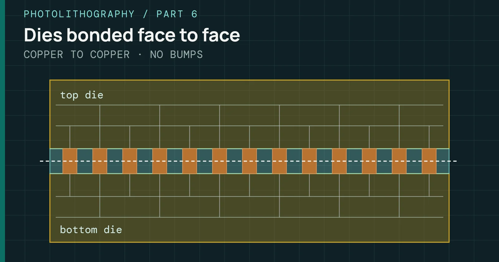
Figure 3.11 shows the three side by side. In a wire-bonded stack the dies sit offset so each die’s edge pads stay reachable. TSVs run straight through the silicon, which gives a shorter path and higher data rates between stacked dies; Toshiba’s 2015 sixteen-die prototype passed over 1Gbps. Wire bonding was the prior art for stacked NAND, and the patents treat it as the baseline. Offsetting each die exposes its pads for one bonding pass, and one sets a 24-die wire-bonded package against an 8-die stack. The third panel is a different level. Inside one die, bonded designs build the array and the logic on separate wafers and join them.
Supply voltage and binning
NAND needs two supplies, a core supply for the array and a separate I/O supply (VccQ) for the interface to the controller. The I/O supply has dropped as the interface sped up, and controllers that pair with both older and newer NAND support both levels. As of October 2026, Open NAND Flash Interface (ONFI) 4.0 introduced NV-DDR3 with VccQ at 1.2V, and the NV-LPDDR4 interface in ONFI 5.2 also runs at 1.2V. ONFI 6.0, published in January 2026, drops the NV-DDR3 definition from the spec and extends NV-LPDDR4 to 4,800MT/s. Marvell’s 88NV1160, for example, lists VccQ at 1.2V and 1.8V. Part 5 covers how the board delivers each rail.
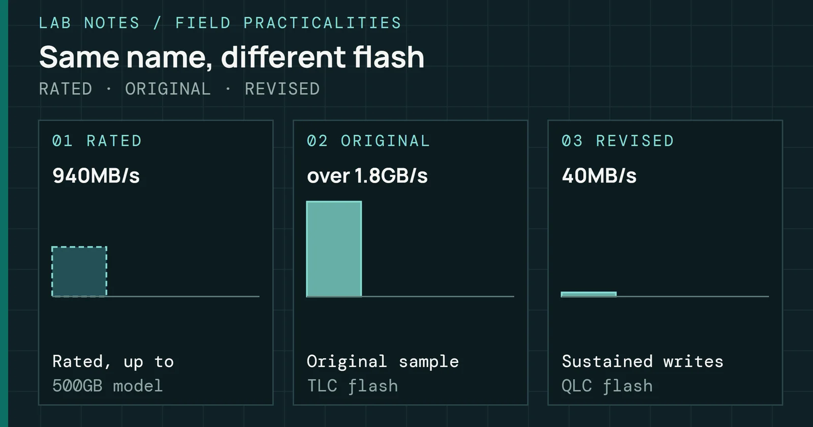
Fabs test every die and sort by quality. One patent describes the usual practice as bins by usable density, with Bin 1 for more than 95% of blocks usable, then 90%, 85% and 75%, with any chip below Bin 1 called a downgrade chip. A lower bin means a die that works but carries more factory bad blocks. From the outside, two drives with the same model number, bought months apart, can carry different NAND. Documented swaps changed the NAND type, and a grade-only change would be harder to catch. That is a procurement and field reliability problem. Part 4 covers the NAND supply side, and The Field Practicalities covers a real case with the Crucial P2.
NAND timing parameters: the physics made measurable
Every layer in the hierarchy has a clock, and the controller has to respect it. Otherwise the operation fails or comes back dirty. Three array times matter most. They are tR (sense a page into the page register), tPROG (program a wordline) and tBERS (erase a block).
NAND timing parameters: the physics made measurable
Erase takes the longest, so it sets the floor for GC latency
Datasheet ranges on a log time axis
Figure 3.12 puts the three on one log axis. They differ by orders of magnitude. A die that is busy with an erase cannot serve a read until the erase ends or is suspended, so the longer the operation, the longer the tail it can add.
Datasheets and the ONFI spec give the ranges in the table, along with what each parameter controls. Datasheet values vary by part. Micron’s 3D NAND flyer, for example, lists a typical tBERS of 15ms, tPROG of 1,300 to 1,630µs and tR of 77 to 100µs across its two parts.
| Parameter | Range | What it controls |
|---|---|---|
| tPROG | 0.2–2ms | Page or wordline program time, one-shot or multi-pass depending on the part, rising with bits per cell. Datasheet maxima run higher |
| tBERS | 3.5–15ms | Block erase time, which sets the latency floor for GC operations |
| tR | 25–150µs | Array sense time, from read confirm until data reaches the page register. The upper end is a datasheet maximum |
| tREA | 16–40ns | RE# access time, from RE# low to valid output data. ONFI maximum by interface mode |
tPROG spans more than an order of magnitude because more bits per cell means more target voltage levels and finer incremental step pulse programming (ISPP)Incremental step pulse programming raises the program voltage a small step with every pulse and checks the cell between pulses, so charge lands precisely. step sizes. A lower page only has to resolve a couple of wide clusters of states. An upper or extra page has to resolve eight or sixteen tight states in the same programming window. The low end, roughly 200µs, is a page programmed in SLC mode. The 2ms end is a QLC wordline resolving sixteen tight states, and a 1Tb QLC part reports 2ms and 110µs. A low-latency 96-layer SLC part described in a JSSC paper sits below the range, with a 75µs program time and a 4µs read.
tR sets base read latency, but tPROG and tBERS are the ones that stretch tails. A page program holds its die for hundreds of µs to a few ms. A block erase takes roughly 3.5 to 15ms, and the host can see that if GC fires without free-block headroom. Firmware hides the waits by interleaving dies on the same channel and suspending programs and erases for reads. These numbers change with wear, as the next section shows.
A die is not a passive array. It carries its own control logic, so the controller issues a command and the die sequences the pulses and verifies behind tR, tPROG and tBERStR is the time to read a page into the buffer, tPROG the time to program a page and tBERS the time to erase a block. Erase is slowest. on its own. One 4Gb part put a Bose-Chaudhuri-Hocquenghem (BCH) error-correction engine on the die that corrects up to 5 bits per codeword, and a survey of flash architecture describes the on-die blocks and test modes. Designs typically repair bitlines before the controller sees the die. Spare columns replace defective bitlines at wafer sort, and the repair data loads at power-on. NAND typically has no spare rows, so a wordline short takes the whole block out. Factory bad blocks are the defects that repair cannot fix, and Part 6 covers how firmware handles them.
How timing parameters shift with wear
Fresh NAND erases near the fast end of the spec. Oxide is intact, charge trapping is consistent, and erase completes in one loop. As P/E cycles accumulate, firmware has to spend more time to get the same confidence.
Program time behaves differently from erase time. In planar characterization, worn oxide passes charge more easily, so cells reach verify in fewer ISPP steps. Grupp and colleagues measured program time falling by nearly 50% over the life of SLC parts and by 10 to 15% in multi-level-cell (MLC) parts. I found no measurement of program time against wear on 3D parts, so treat this as planar behavior.
tBERS is the one that moves. An aged block with a dense trap population needs more erase loops at higher voltage to clear residual charge from nitride or oxide that no longer yields to the original voltage. In one 3D TLC characterization, worn blocks needed two or more erase loops where fresh ones needed one, so a 3.5ms erase can take 7ms or more late in life. That matters because tBERS is the GC latency floor. Late-life drives keep a die busy longer per erase, so GC competes harder with host I/O. Tail spikes get worse toward end of life for two reasons. GC runs more often as free-block headroom shrinks, and each erase itself is slower.
A block erase is not a single pulse. In one published planar design it runs as a small program of its own. An optional program-before-erase pass writes every wordline with no verify, stepping from 12V to 17V in 1V steps over about 150µs, so every cell starts from the same programmed state and cells that were already erased are not pushed into deep over-erase. Then up to four erase pulses follow. Each ramps the p-well to about 23V with the wordlines at 0V and lasts about 1,025µs, and each is followed by a hard erase verify. When every cell passes, a program-after-erase step soft-programs the over-erased cells back up, which tightens the erased distribution. A read-all-1 check closes the sequence.
How timing parameters shift with wear
An erase is a short program, not one pulse
One block erase in one published planar design
The sequence also shows what an interrupted erase can leave behind. Cut power after the pre-program and every cell has been pushed toward programmed, with no verify. Cut it during the pulses and the block is partly erased, and some cells can read as erased with little margin. Cut it before the soft program and some cells are over-erased. In every case firmware has to treat the block as dirty and erase it again. These voltages and timings belong to planar NAND. Many 3D designs use GIDL erase, as Part 2 describes, so the numbers differ by vendor.
Read window budget: the margin that wear consumes
NAND wear-out comes down to one margin, and it sits between cell physics and ECC. Every cell type stores charge in voltage bands. TLC has eight states, split by thresholds. Between the upper tail of one distribution and the lower tail of the next lies the read window, the voltage space where the controller can place a reference and still know which state it has. The sum of those gaps is the read window budget (RWB)The read window budget is the voltage room left between distributions for placing read references. It shrinks with every added bit per cell and every cycle of wear., the margin left before adjacent distributions overlap and classification becomes a guess. This series uses the term for the total margin across all the states.
A fresh TLC block has tight clusters and real gaps, so RWB is large and error rates stay low.
Read window budget: the margin that wear consumes
Wear widens each state until the gaps between neighbors close
Eight triple-level-cell states, fresh and worn
In Figure 3.14 the dashed curves are fresh cells and the solid curves are worn cells. Where neighboring solid curves cross a read reference, the shaded overlap is cells that read as the wrong state. Those are bit errors, and ECC cleans them.
P/E cycling broadens the tails, as Part 2 shows. Keep wearing and the misclassification rate climbs, RBER rises, and eventually a codeword holds more errors than ECC can fix. It is uncorrectable. So wear-out error growth tracks the P/E count instead of arriving at random. RWB narrowing is a function of P/E, retention age, temperature, and read disturb. Controller ECC is sized to the RBER expected at the rated end-of-life P/E count, which is the point where the worst blocks hit minimum viable RWB under the rating’s workload and retention assumptions. Read retry is the response when the standard read reference no longer sits in a usable gap, and Part 8 covers how the controller walks alternate thresholds until one fits.
The field catch is that RWB does not shrink evenly. Upper pages cross the most references, so they hit the ECC wall first. High-wear blocks go faster than low-wear ones. Hot regions go faster than cool ones. When an aged drive shows errors clustered in specific logical block address (LBA)A logical block address numbers the fixed-size blocks the host sees, starting at zero. The drive decides where each one is physically stored. ranges, you are usually looking at data written and aged together. Which physical region that is depends on the FTL, because the LBA only names the data.
Reading errors by page type and landing pattern
The page type an error came from tells you more than the error itself. When a read fails or needs multiple retries, the physical location (which wordline, and which page type on it) is context the NVMe Error Information log does not spell out. Neither does the standard health log. Vendor-specific logs and telemetry sometimes do. Three cases cover most of what an uncorrectable read can mean.
Reading errors by page type and landing pattern
Where the failure sits tells you which causes to rule out first
Three cases for an uncorrectable read
Read the tree from the top. An uncorrectable on an upper page at high P/E is expected wear. The upper page was programmed into tight margins for thousands of cycles, and ECC headroom ran out. This is the designed end-of-life case for the block. Firmware should have been watching RBER and relocating first, but the failure itself is not strange. An uncorrectable on an upper page at low P/E is not. Either that block took more cycles than the drive-level P/E shows, it ran hot enough to accelerate retention loss, or there is a process defect in that region, and each explanation wants a different response.
Lower-page failures carry the most weight. Under 1-2-4 coding, LP has the fewest references to cross and the lowest error rate. Read disturb moves the erased and lowest programmed states first, and those boundaries belong to the upper page, so ordinary disturb fails upper pages first. An LP failure at moderate wear with clean upper pages most often points to a defective region with severe oxide damage. Alongside upper-page failures on the same wordline, an LP failure points to a shift large enough to cross the middle reference, such as a long power-off or read disturb that beat the refresh threshold.
Pull the full NVMe error log and the health log first. Then correlate the failure with Percentage Used and Media and Data Integrity Errors (Part 8 defines both), plus power-off time pulled from asset records. If sustained write throughput is sliding faster than small changes in spare and media errors would explain, lost multi-plane alignment from retired blocks is a candidate.
Landing pattern matters as much as the NAND type. How firmware uses the page hierarchy shows up as different behavior between drives and between deployments. Drives that park write-hot metadata in SLC-mode blocks and move data off high-wear blocks early can keep a lighter ECC load. A drive with a smaller SLC cache, a pool of blocks programmed one bit per cell as a write buffer that Part 6 covers, and higher WAF may accumulate upper-page errors faster under the same host traffic.
Every block programs wordlines in a vendor-fixed order, and multi-pass parts also fix the page order within each wordline (LP to MP to UP to XP), whatever the host pattern is. Sequential work keeps blocks mostly valid until they get erased, so the ECC load spreads evenly. Random small writes land in open blocks the same way, but they invalidate data across many blocks, so GC copies more pages and WAF climbs. Under sustained random writes, WAF piles more P/E cycles onto every host byte, so the share of the NAND at high upper-page error rates grows faster than under sequential writes. That WAF gap is the real reason random-write endurance and sequential-write endurance are different numbers.
When a replacement drive behaves worse than the failed unit, the answer is often the landing pattern rather than the silicon. Say the original spent years on sequential writes and the replacement sees mixed random traffic at the same rate. That replacement will burn P/E cycles faster through higher WAF and spend its upper-page ECC headroom sooner, on the same NAND.
Wear also shows as timing. A fleet whose tail latency drifts up over months with no workload change may be showing the wear curve as timing, once fill level, firmware, and thermals are ruled out. The p99.9 and p99.99 latencies (Part 9 defines them) tend to show it first, because reads stuck behind erases and retries on the weakest blocks land there before the median moves. ioTraX can log each drive’s average read and write latency to CSV alongside throughput, IOPS, and I/O size, so a slow drift can be lined up against the workload over a long run. It records an average per sample and no percentiles, so the tail itself needs another source.
What the hierarchy hands to 3D stacking
On a real drive, the hierarchy shows up as latency spikes behind an erase, errors that cluster in upper pages, and sustained throughput that scales with die count rather than with the interface number on the spec sheet.
What the hierarchy hands to 3D stacking
From Cell to Die feeds 3 later parts.
Arrows run to the parts that build on this one.
Figure 3.16 marks Parts 4, 7 and 8 as the later parts that build directly on this one. Part 7 builds garbage collection on the page and block asymmetry, and Part 8 builds read retry on the read window.
Part 4 shows what happened when planar NAND ran out of room, and how this same hierarchy works once the industry stacks cells through hundreds of layers.
Sources
Primary is the original paper, standard or datasheet. Secondary is a review, a vendor summary or a news report. Measured is my own test data.
Show all 39 sources, 30 primary
- PrimaryNew ultra high density EPROM and flash EEPROM with NAND structure cellIEEE Xplore (IEDM 1987, Masuoka et al.), 1987
- PrimaryUS5657270A - Electrically erasable programmable read-only memory with threshold value controller for data programmingGoogle Patents, 1995
- PrimaryUS7286408B1 - Boosting methods for NAND flash memory - Google Patentspatents.google.com, 2006
- PrimaryCharacterizing Flash Memory:Anomalies, Observations, and ApplicationsMICRO, 2009
- PrimaryInside NAND Flash MemoriesSpringer, 2010
- PrimaryMicron TN-29-19, NAND Flash 101 (Rev. B, 2010)Micron Technology, Inc., 2010
- PrimaryUS8502368B2 - Multi-chip package with offset die stackingGoogle Patents, 2013
- PrimaryRead Disturb Errors in MLC NAND Flash Memory: Characterization, Mitigation, and RecoveryIEEE/IFIP DSN, 2015open copy
- PrimaryThree-Dimensional 128 Gb MLC Vertical NAND Flash Memory With 24-WL Stacked Layers and 50 MB/s High-Speed ProgrammingIEEE Journal of Solid-State Circuits, vol. 50, no. 1 (IEEE Xplore), 2015
- PrimaryMicron 3D NAND flyerMicron, 2016
- PrimaryVulnerabilities in MLC NAND Flash Memory Programming: Experimental Analysis, Exploits, and Mitigation TechniquesHPCA, 2017
- PrimarySilicon Motion SM2262EN/SM2262 product briefSilicon Motion, 2018
- Primary13.5 A 128Gb 1b/Cell 96-Word-Line-Layer 3D Flash Memory to Improve Random Read Latency with tPROG=75μs and tR=4μsISSCC, 2020
- PrimaryA 1.33-Tb 4-Bit/Cell 3-D Flash Memory on a 96-Word-Line-Layer TechnologyIEEE Journal of Solid-State Circuits, 2020
- PrimaryNot-So-Solid State: SSD Makers Swap Parts Without Telling UsTom's Hardware, 2020
- PrimaryA 128Gb 1-bit/Cell 96-Word-Line-Layer 3D Flash Memory to Improve the Random Read Latency With tProg = 75 μs and tR = 4 μsIEEE Journal of Solid-State Circuits, 2021
- PrimaryUnsavory Flash Swap: Re-Testing Crucial’s P2 SSD After QLC DowngradeTom's Hardware, 2021
- PrimaryAERO: Adaptive Erase Operation for Improving Lifetime and Performance of Modern NAND Flash-Based SSDsACM ASPLOS, 2024open copy
- PrimaryONFI 5.2 specificationONFI, 2024
- PrimaryDesign Tradeoffs for SSD PerformanceUSENIX
- PrimaryEndurance of NVMe, SAS, and SATA SSDsSNIA
- PrimaryError Characterization, Mitigation, and Recovery in Flash-Memory-Based Solid-State Drivesopen copy
- PrimaryError Characterization, Mitigation, and Recovery in Flash-Memory-Based Solid-State Drives
- PrimaryFrontgrade UT81NDQ512G8T: 4Tb TLC NAND Flash datasheet
- PrimaryMarvell 88NV1160: PCIe Gen3x2 NVMe DRAM-less BGA SSD Controller product brief
- PrimaryONFI 2.0: Open NAND Flash Interface Specification, Revision 2.0
- PrimaryONFI specificationsONFI
- PrimaryReducing SSD Read Latency via NAND Flash Program and Erase SuspensionUSENIX
- PrimaryToshiba Develops World’s First 16-die Stacked NAND Flash Memory with TSV TechnologyKioxia Singapore Pte. Ltd.
- PrimaryUT81NDQ512G8T 4Tb TLC NAND Flash datasheetFrontgrade
- SecondaryUS20100017556A1 - Non-volatile memory storage system with two-stage controller architectureGoogle Patents, 2009
- SecondaryUS20130119542A1 - Package having stacked memory dies with serially connected buffer diesGoogle Patents, 2012
- SecondaryInside Solid State Drives (SSDs), Second EditionSpringer, 2018
- SecondarySamsung 980 M.2 NVMe SSD Review: Going DRAMless with V6 V-NAND (Updated) (Tom's Hardware, by Sean Webster)Tom's Hardware, 2021
- SecondaryMicron Ships World's First 232-Layer NAND, Extends Technology LeadershipMicron Technology, Inc., 2022
- SecondarySemiconductor Memories and SystemsWoodhead Publishing (Elsevier), 2022
- SecondaryJEDEC e.MMC standard pageJEDEC
- SecondaryScalable Wordline Shielding Scheme using Dummy Cell beyond 40 nm NAND Flash Memory for Eliminating Abnormal Disturb of Edge Memory Celliopscience.iop.org
- SecondarySK hynix H25GTD0 321-layer V9 1 Tb TLC 3D NAND process flow analysis (TechInsights)