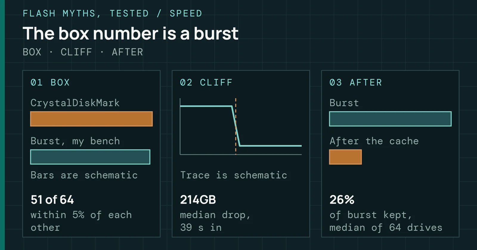
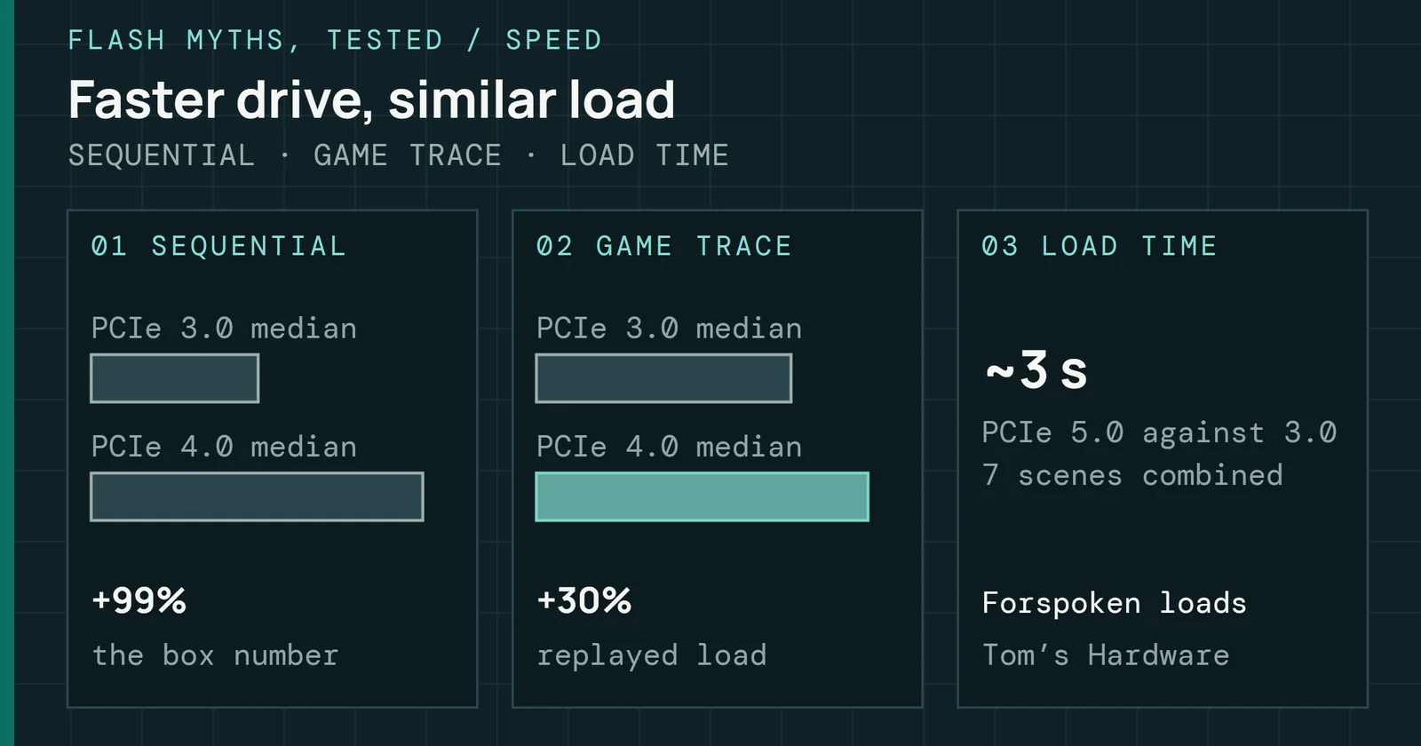
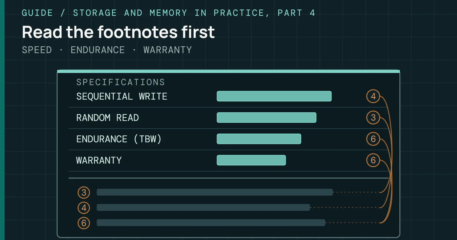
While the storage industry races to print bigger sequential numbers on retail packaging, the gap between marketing promise and daily reality continues to widen. A Gen5 drive claiming 14,000 MB/s sounds like the future, until you realize your operating system boots at QD1, your applications launch with random 4K reads, and that box number was measured on an empty drive at a queue depth no consumer workload will ever touch. That spec sheet is a best-case scenario engineered in a vacuum, and the road is something else entirely.
Benchmarking 101
SSD Benchmarking 101, Part 1: A Repeatable Test Method
Build a repeatable SSD test method: control the host, precondition the drive, and understand cache behavior, queue depth, and workload mix.
On this page 20 sections
This guide exists because I spent years learning that difference firsthand. Tests on empty drives produced published numbers no user would ever see. Without pre-conditioning, QLC silicon posted TLC-tier speeds for the first ten gigabytes before falling off a cliff. With Windows Search Indexing left on, I spent two days chasing a phantom IOPS spike that turned out to be the OS reading my test files before I could. Each of those became a methodology rule. Every rule became a section of what you are reading now.
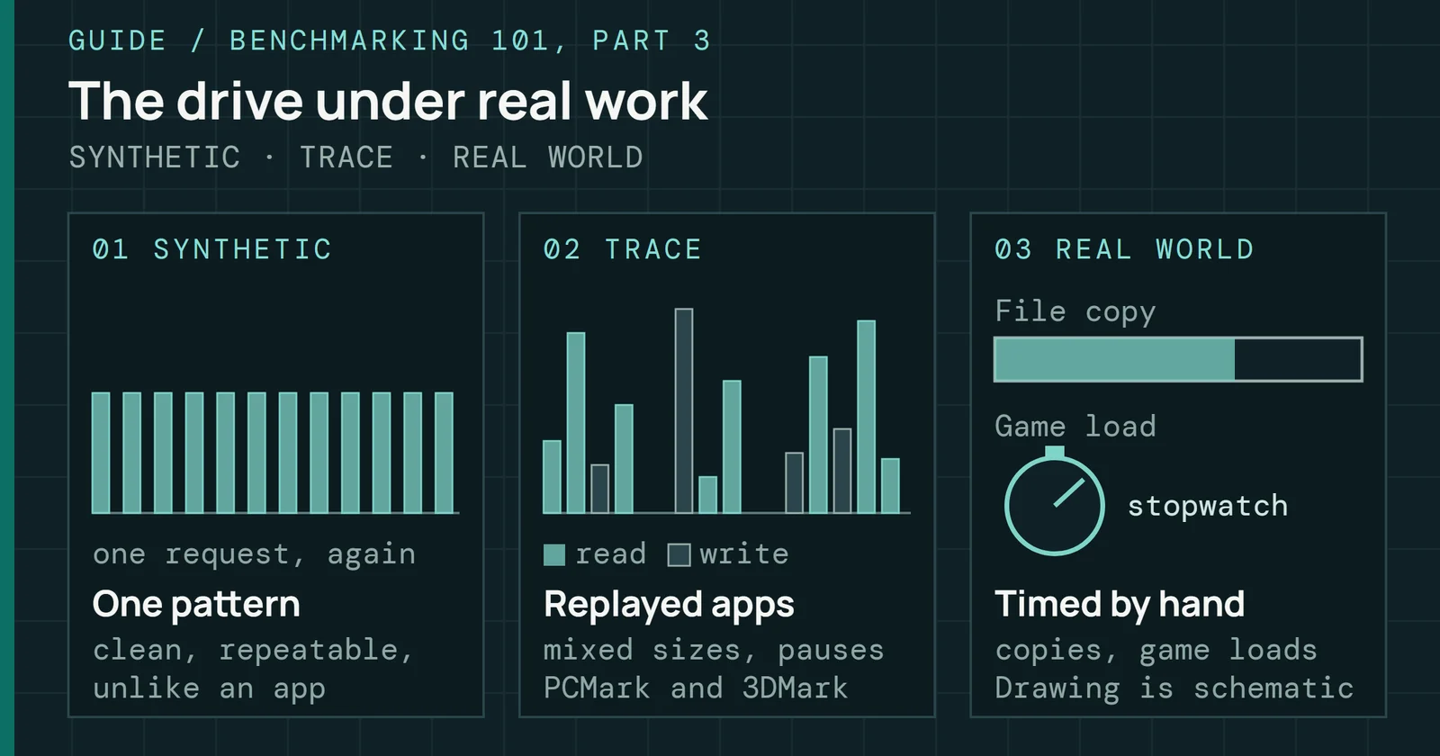
This is Part 1 of Benchmarking 101, the framework behind every review, built from hundreds of drives tested across every category from budget QLC SATA units to flagship Gen5 NVMe platforms. It answers one question: what has to be true of the host, the drive and the workload before a number means anything? Part 2 covers the synthetic tools, and Part 3 covers application and trace-based tests.
Methodology: the system lockdown
The single greatest enemy of an accurate SSD benchmark is the operating system sitting between you and the silicon, more than the drive itself. By design, Windows is a chaotic environment. Background telemetry pulses, Search Indexing crawls through your test files, Defender scans every write, and TRIM commands fire on schedules you never set. Before you can measure a drive’s performance, you must first silence everything that would contaminate the measurement. I call this the Lockdown Protocol, and it’s non-negotiable.
Methodology: the system lockdown
Six host controls are fixed before the first data point
A professional test bench is a controlled experiment. Nothing changes between runs except the variable you are measuring. That sounds simple until you realize how many variables Windows introduces without asking. Not to mention the various Linux distros and macOS. These controls must be confirmed before a single data point is recorded.
| Control | Required State | Consequence of Failure |
|---|---|---|
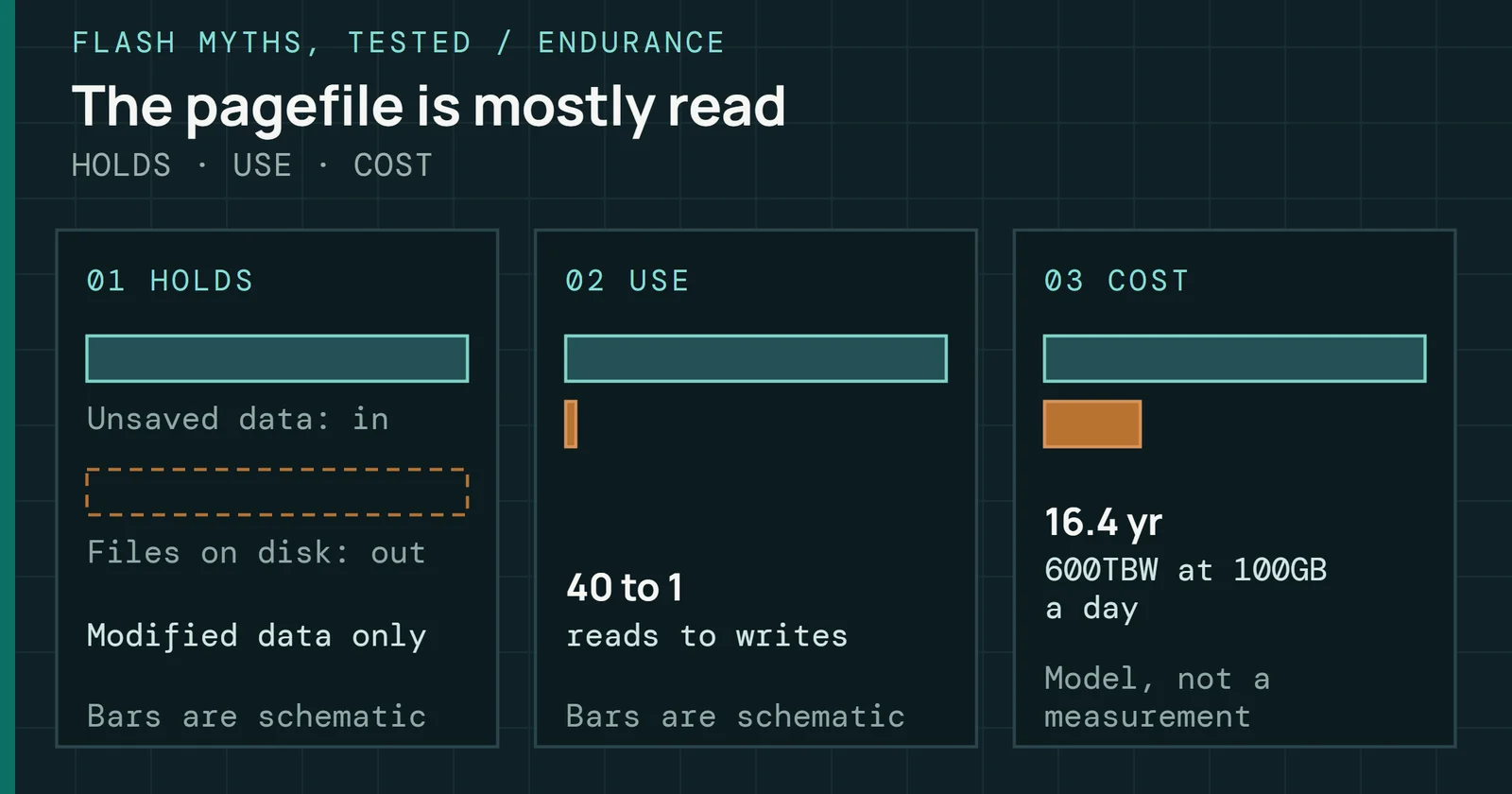
| Drive Under Test (DUT) | Mounted as secondary volume, never the boot drive | OS pagefile writes and log activity inject latency spikes into random read data |
| Anti-virus | Disabled or DUT excluded | Real-time scanning triggers random I/O bursts that corrupt sequential write measurements |
| Search Indexing | Disabled for DUT volume | Indexer reads test files before you do, inflating read cache hits and skewing IOPS |
| Power Plan | High Performance, PCIe ASPM off | Link state power management adds microseconds of wake-up latency to every I/O request |
| Background Services | Updates paused, telemetry minimized | Scheduled tasks can spike CPU and disk I/O mid-test without warning |
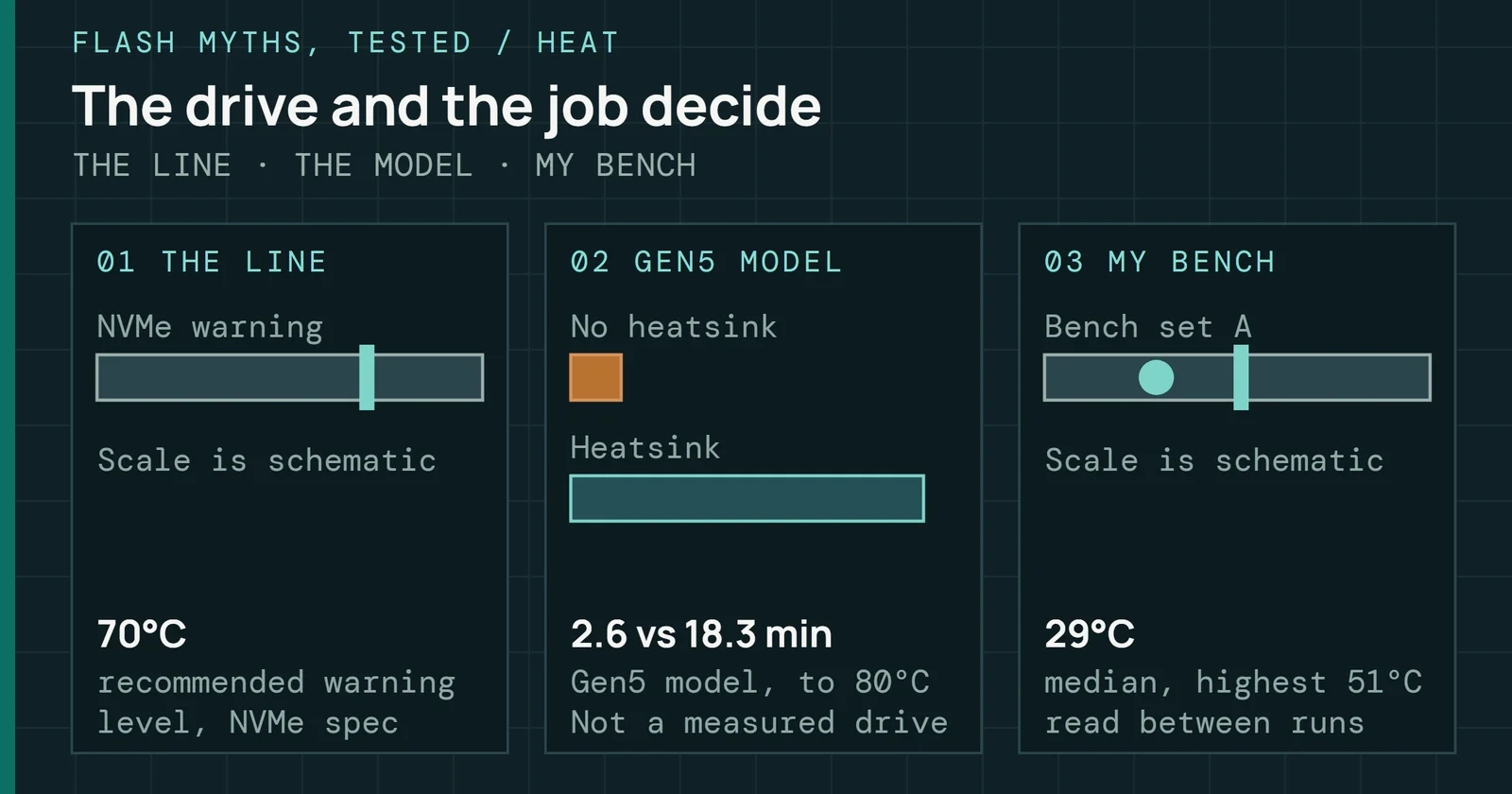
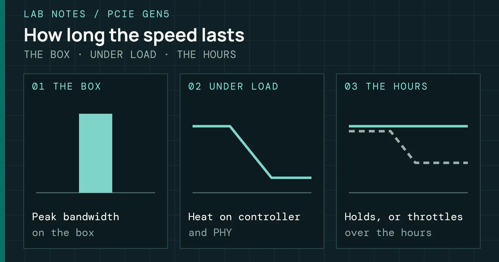
| Thermal Baseline | Ensure DUT temps remain under throttle range | When testing, thermals can wreak havoc on test results. Actively cool the drive to isolate. |
| Why This Matters: If you run the same test three times and get three different numbers, your system is not locked down. Repeatability is the minimum standard. Without it, your data is anecdotal, not analytical. |
The “dirty drive” reality
Testing an empty SSD is like benchmarking a sports car on a treadmill. Every number looks spectacular and tells you nothing about the road. A fresh-out-of-box drive has pristine NAND pages, an empty Flash Translation Layer, and a fully available SLC cache. Call it the silicon equivalent of a clean room. No consumer will ever experience this state for more than a few hours after unboxing, yet it is the state that produces every number on the spec sheet.
The “dirty drive” reality
A used drive is a different device from a fresh one
Your reader’s drive is dirty. Half-full. Its FTL tables are populated with mapping entries. Its garbage collection engine is running in the background, recycling stale blocks while trying to service new requests. Its SLC cache has been partially consumed and may not have fully recovered from the last large write. That is the drive you need to benchmark, because that is the drive that determines whether the user perceives their system as fast or slow.
Pre-conditioning
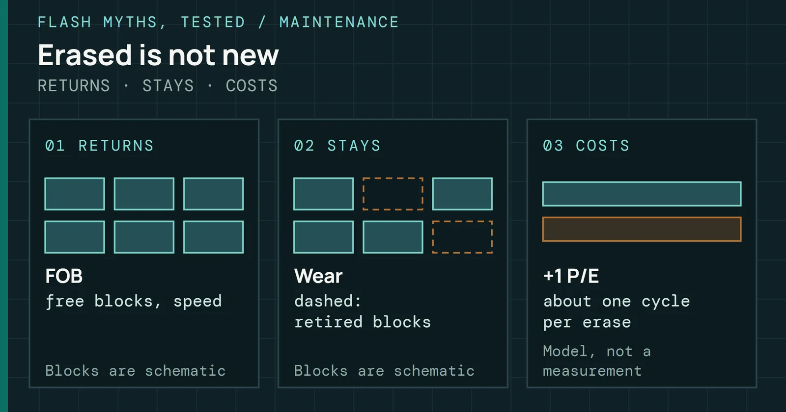
Before any benchmark suite begins, the DUT must be moved from its Fresh-Out-of-Box (FOB) state to a realistic Used State. Running a full-span sequential write pass does the job, forcing the controller to populate its FTL mapping tables and begin managing wear-leveling across all NAND dies.
Pre-conditioning
A full-span write moves the drive out of its fresh state
Full-span write
Write the entire addressable capacity of the drive at least once before testing begins. That’s the minimum needed to move all NAND blocks out of their erased (FOB) state and force the controller into its steady-state management mode.
The 50% fill rule
Reviewers such as PCPartPicker benchmark drives at 50% capacity. Its published method fills the first 50% of the disk before its read tests, and it resets the drive to fresh-out-of-box before each write run, unlike the full-span pass above. My reasoning for filling the drive is that it forces the controller to perform real-time garbage collection and wear-leveling while simultaneously servicing your test workload. An empty drive can defer all of that housekeeping, and deferred housekeeping produces flattering numbers that evaporate the moment the user fills the drive.
SLC cache behavior
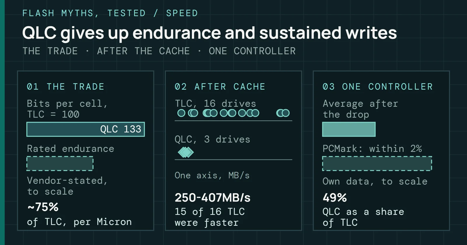
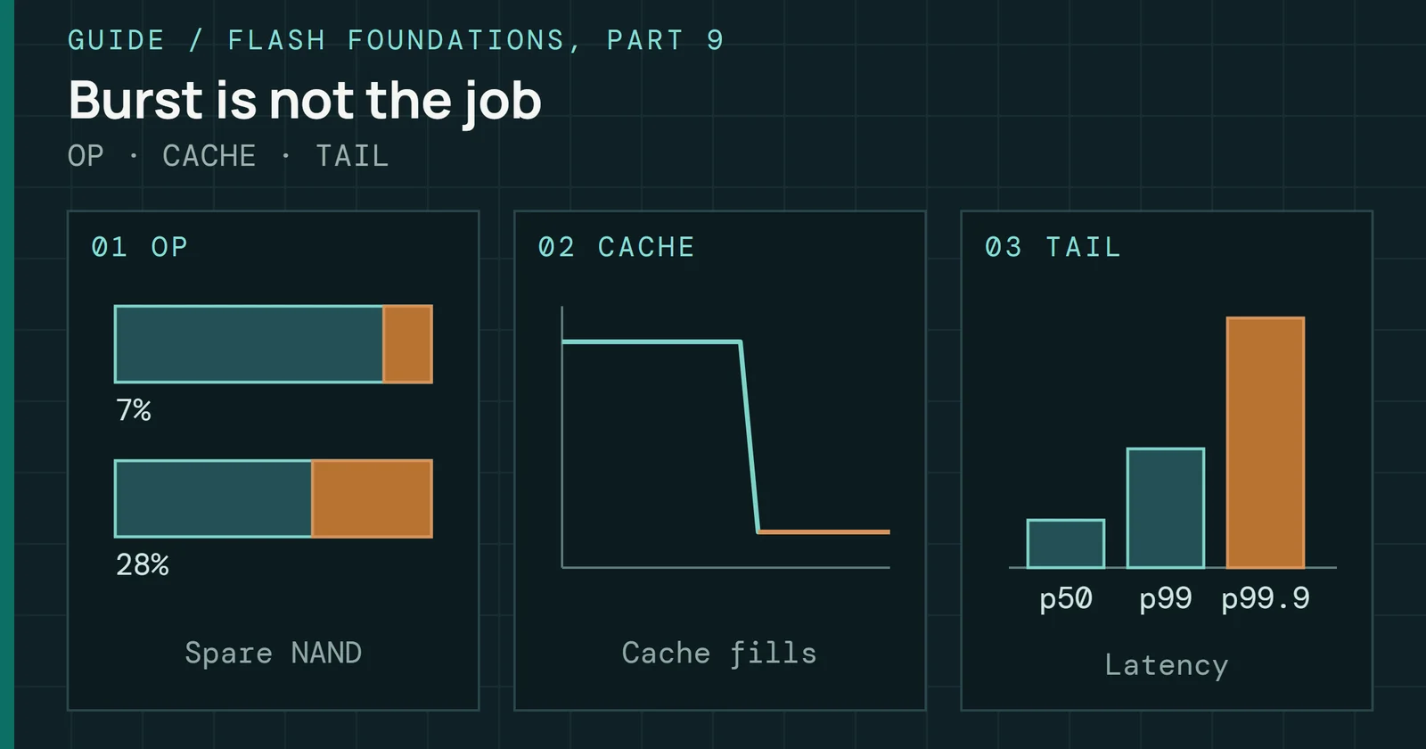
Nearly every modern consumer SSD (TLC and QLC alike) uses a portion of its NAND in a pseudo-SLC mode to absorb burst writes at high speed. That region is the SLC write cache, the single most important architectural detail for honest benchmarking. Understanding it is the difference between measuring a drive’s marketing performance and its real performance.
SLC cache behavior
Write speed falls sharply once the SLC cache runs out
Cache size
Varies by drive and by fill level. Can be static (fixed GB), dynamic (scales with free space), or hybrid. A 2TB QLC drive might have 200GB of dynamic SLC cache when empty but only 20GB when 80% full, a 10x reduction that transforms the drive’s write personality entirely.
The cliff
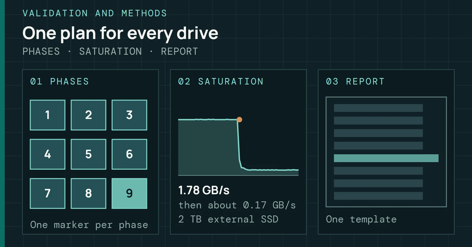
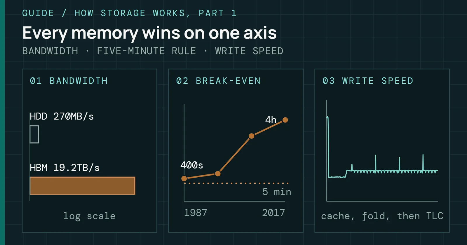
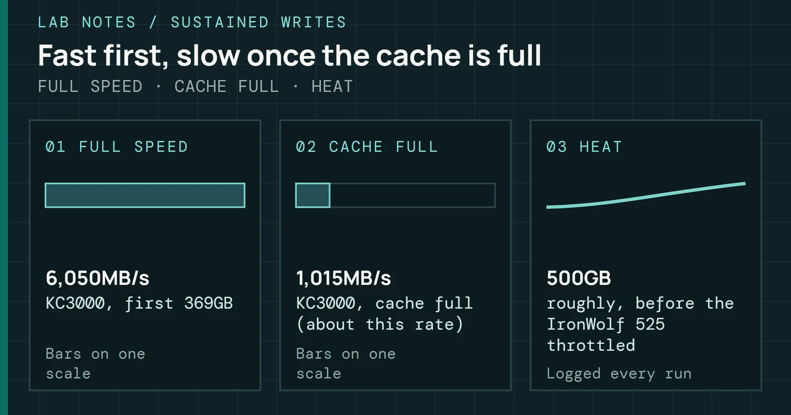
Once the SLC cache is exhausted, write speeds drop to the raw folding speed of the underlying NAND. In one modeled example of a QLC drive, speed falls from 5,000 MB/s to under 500 MB/s. That is a 90% collapse in a fraction of a second. This post-cache speed is the number consumers actually experience during large file transfers, and it is the number that belongs in your review.
Cache recovery
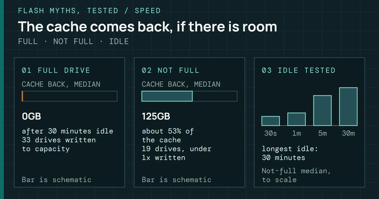
After a heavy write test, the controller needs idle time to fold data from SLC pages into TLC/QLC blocks. That folding is part of garbage collection, and it consumes controller resources. If you run the next test immediately, you are benchmarking a controller that is still doing housekeeping, much like testing a runner mid-sprint.
| The Recovery Rule: Allow 15–30 minutes of idle time between heavy sequential write passes. This ensures the SLC cache has fully recovered and garbage collection is complete. Without this, your next run measures a tired controller, not a rested one, and the difference can be enough to change your conclusion. |
The static data problem
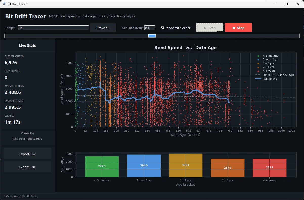
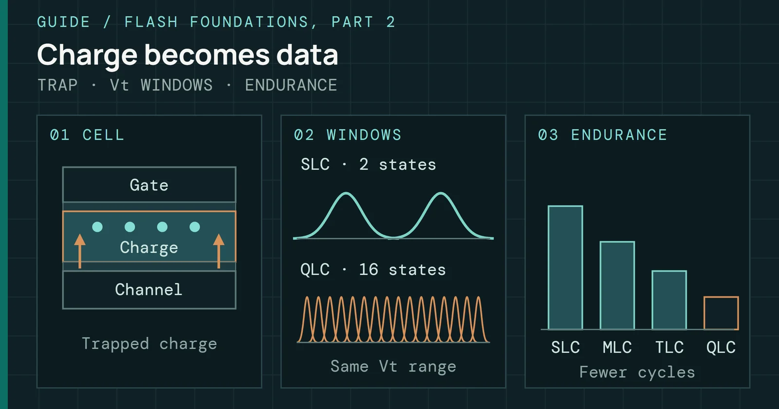
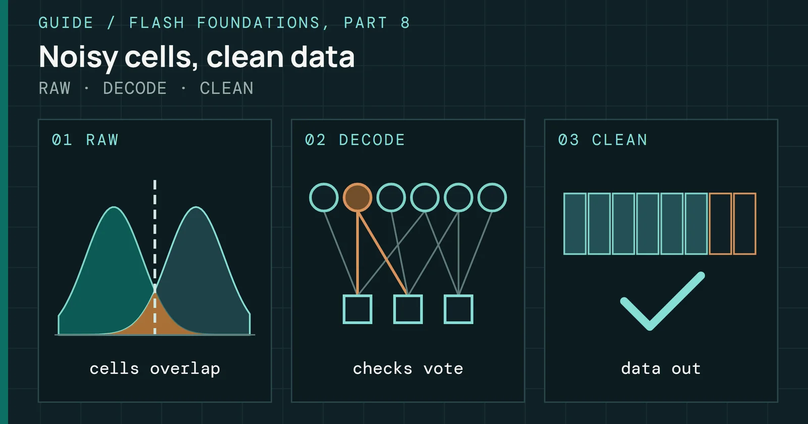
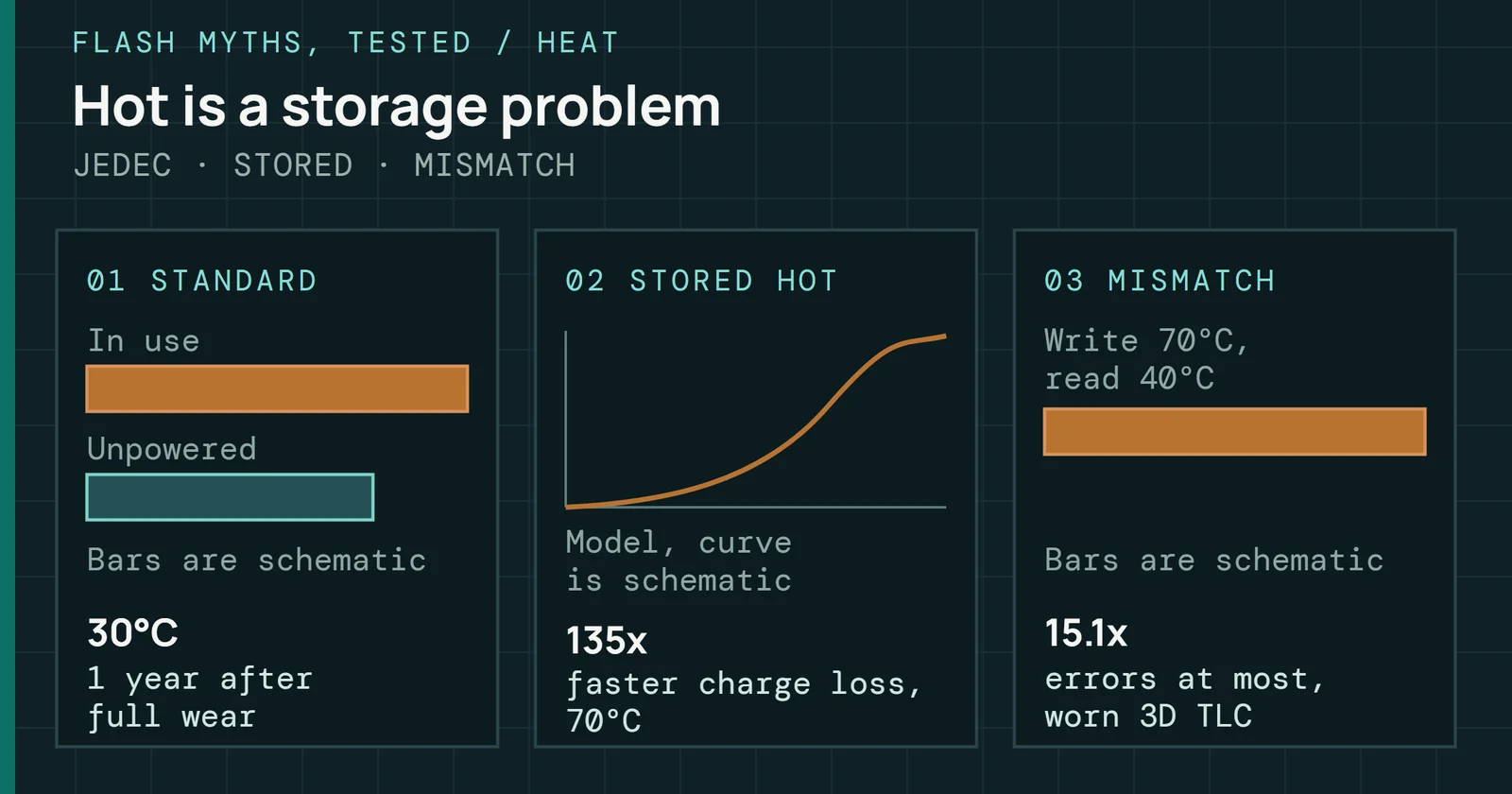
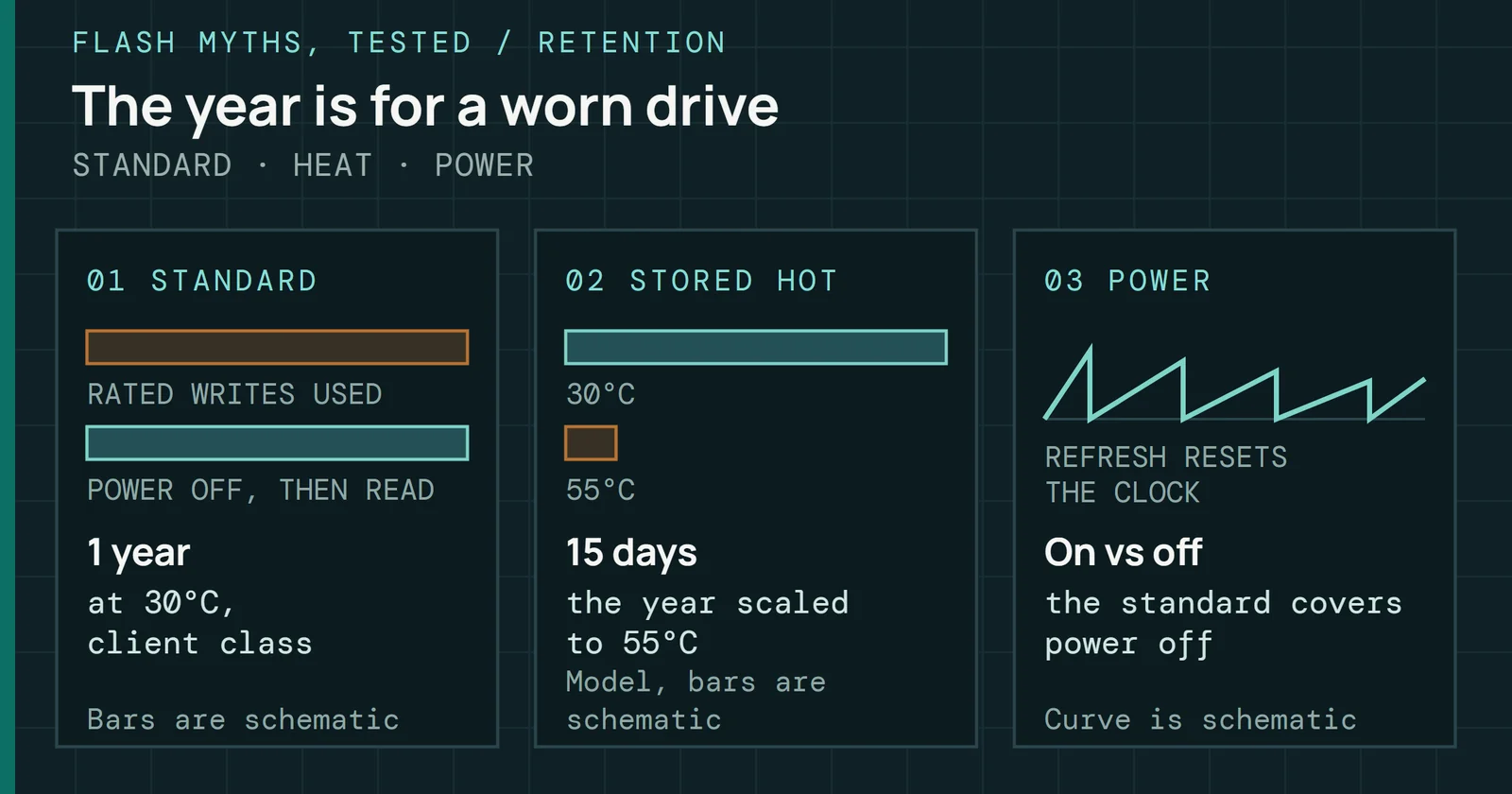
Data folded from SLC cache into native TLC or QLC pages does not maintain its read performance forever. Flash cells store data as trapped electrical charge, and that charge begins dissipating the moment it is programmed. On TLC and QLC, where voltage margins between states are already razor-thin, even modest drift forces the controller to retry reads or invoke heavier error correction. Stale data therefore reads with measurably higher latency.
The static data problem
Old data reads more slowly, so rewrite test files first
I found this when re-reading source files from a test drive that had sat idle for several weeks. Sequential reads on static data had dropped noticeably compared to freshly written files on the same drive. Those cells hadn’t failed, but the charge had drifted enough that the controller was working harder to interpret it.
Enterprise drives handle this with automatic background data refresh cycles, which most consumer drives don’t have. If you’re benchmarking read performance on pre-loaded data, the age of that data affects your numbers. Control for it or document it. I tend to rewrite source datasets before using them in benchmarking runs.
Understanding the variables
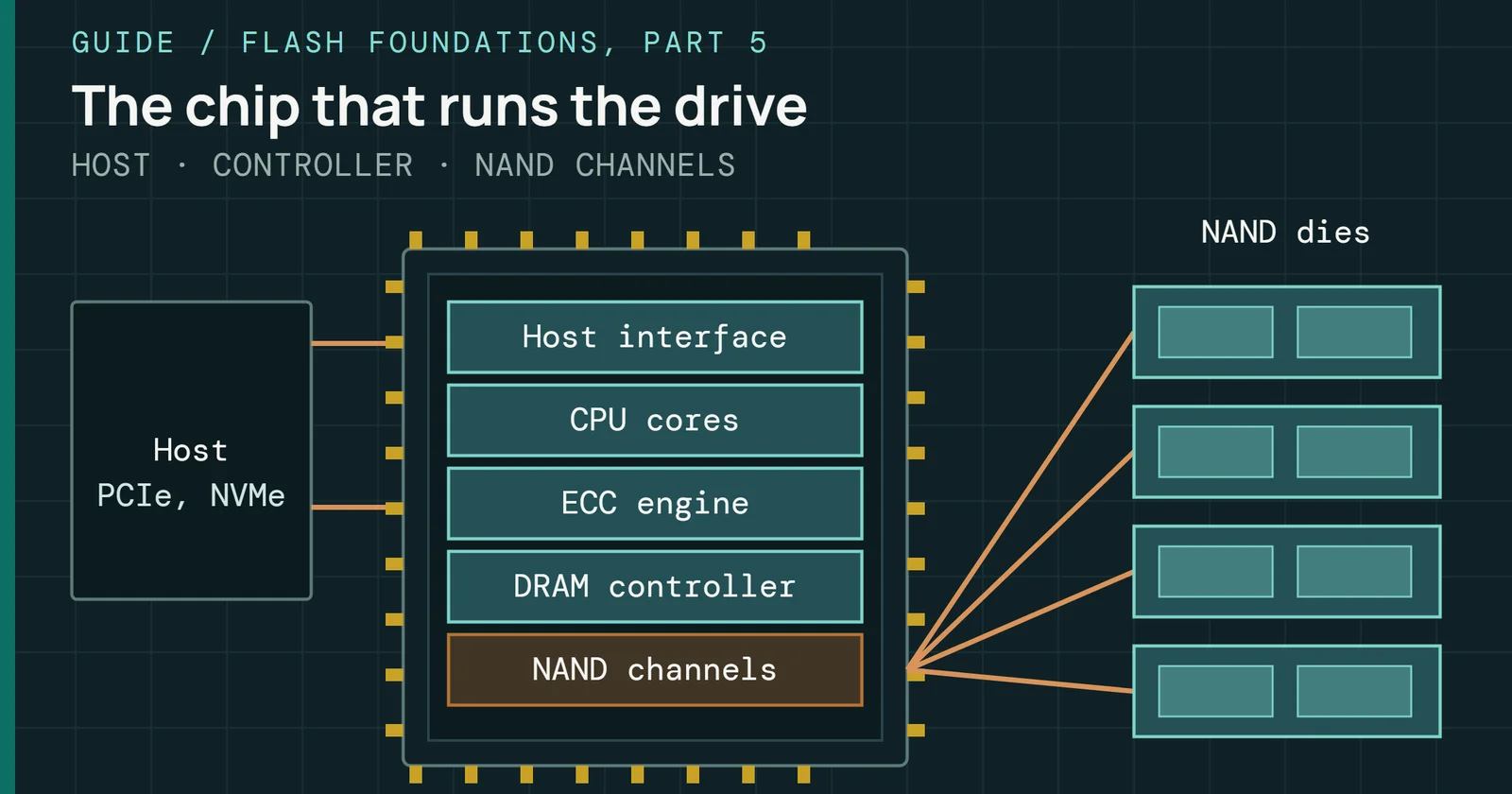
When you see a dip in a performance graph, you need to know which variable caused it. SSD performance is a three-way negotiation between controller logic, NAND physicality, and firmware tuning, and every benchmark you run manipulates at least one of those dimensions.
Understanding the variables
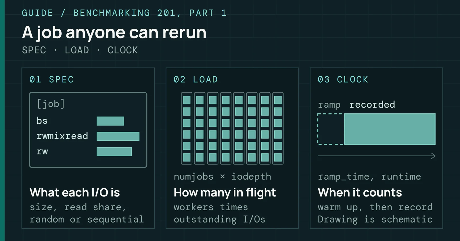
Queue depth times thread count sets the outstanding I/O
I/O request
Single read/write operation issued to storage. Each carries fixed overhead (queuing, controller dispatch, NAND access); fewer/larger requests reduce overhead vs many/small ones for the same throughput.
Block size
The amount of data in each I/O request determines which part of the storage pipeline you are stressing. A 4K read request tests the controller’s ability to locate and return a single page from NAND as fast as possible. A 1M read request tests its ability to stream contiguous data across all channels simultaneously, so the same drive and controller face a fundamentally different workload.
Queue depth (QD)
The number of outstanding I/O requests the controller is juggling simultaneously. Think of it as the length of the waiting line at a deli counter. More requests in the queue means the controller can optimize scheduling and parallelism across its internal channels.
Thread count (T)
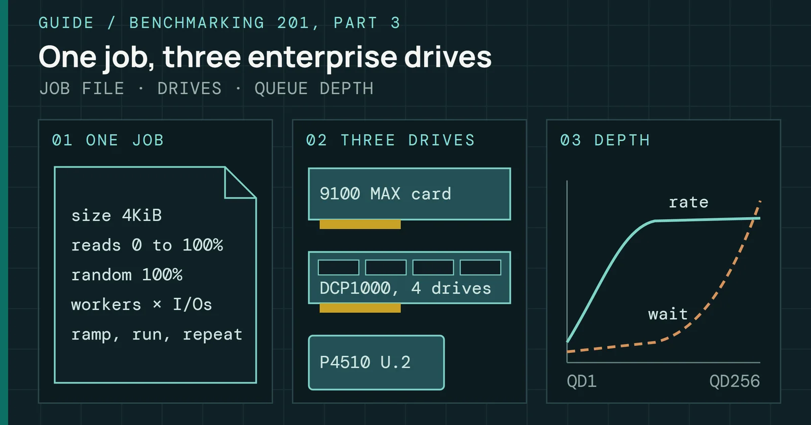
The number of independent processes generating I/O requests. Think of these as multiple cashiers, each with their own customer line. The total outstanding I/O equals the queue depth (QD) multiplied by the thread count (T). For optimal performance, scale threads alongside QD until all CPU cores are effectively utilized. For instance, using 16 threads instead of 2 or 4 in a QD 128 workload can deliver higher performance, particularly at lower QDs, where additional thread parallelism helps sustain higher I/O rates.
Read/write mix
No real workload is purely reads or purely writes. A typical desktop session runs roughly 70/30 read-heavy. Premiere Pro exports with scratch disk activity can flip to 60/40 write-heavy. Games loading assets while autosaving hit both simultaneously. That ratio matters because reads and writes compete for controller resources, and some controllers handle that competition far worse than their isolated read and write scores would suggest.
Read/write mix
Reads and writes compete for the same controller and NAND
A drive that posts excellent numbers in CrystalDiskMark’s separate read and write tests can stumble badly when forced to service both at once, because the controller must manage NAND programming (slow, blocking) while servicing read requests (fast, latency-sensitive) on the same silicon. Mixed-workload benchmarks like PCMark 10 and custom iometer/fio jobs expose this behavior, while pure synthetics hide it.
Sequential vs. random access
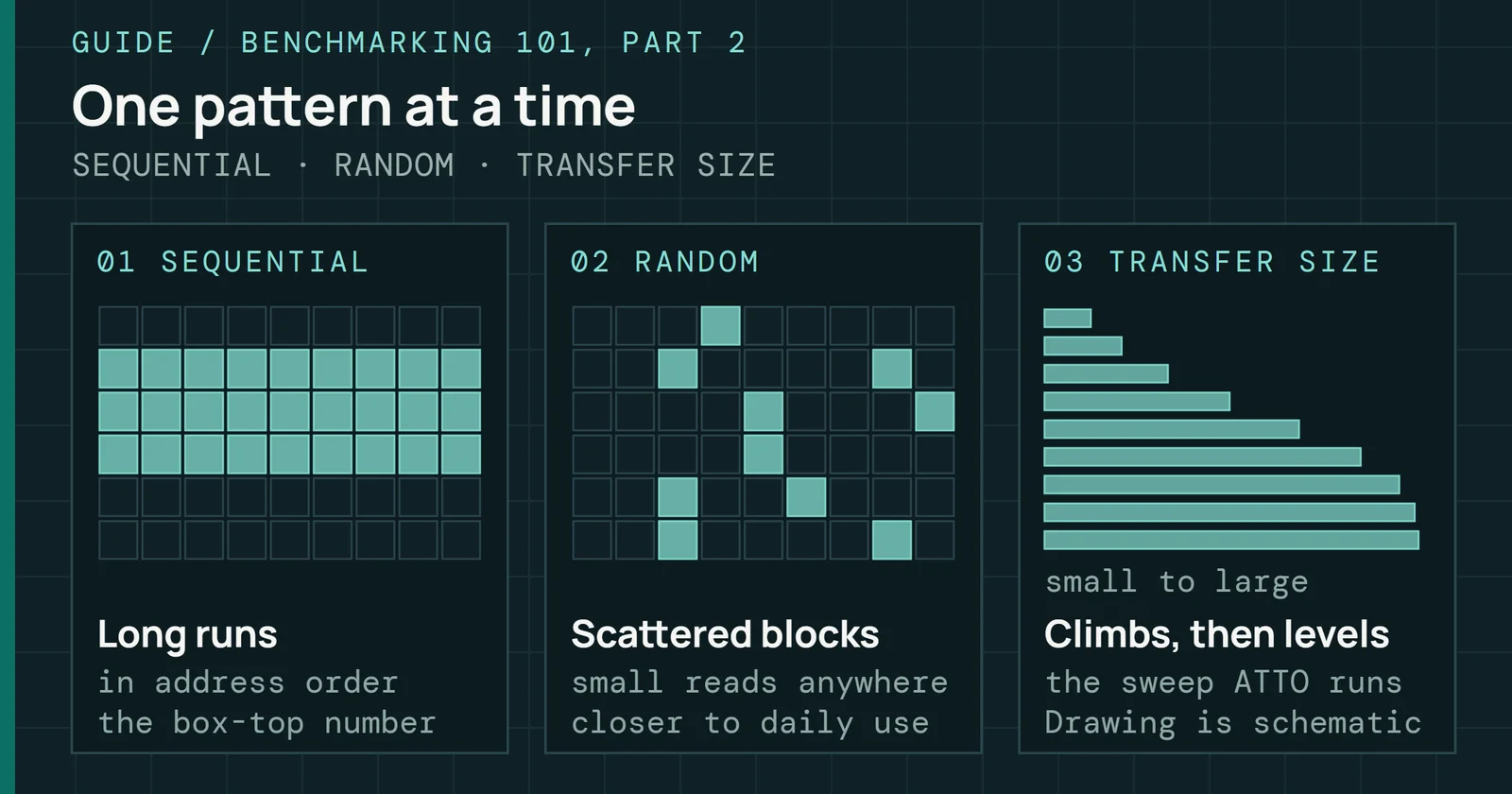
Every I/O request hits either a contiguous address range or a scattered one, and the distinction changes everything about how the controller performs. Sequential access (reading or writing long, contiguous streams) lets the controller prefetch aggressively, pipeline across all NAND channels, and deliver the peak throughput numbers that land on spec sheets. Random access (small requests scattered across the drive’s address space) forces the controller to chase each request individually, with no opportunity to batch or predict what comes next.
Sequential vs. random access
Sequential access batches requests; random access cannot
Between the two, the gap is enormous. A modern Gen4 NVMe drive might post 7,000 MB/s sequential reads but only 60-80 MB/s random reads at QD1. Neither number is a flaw, since sequential I/O plays to the controller’s strengths and random I/O exposes its overhead. For your methodology, what matters is that consumer workloads are overwhelmingly random. OS operations, application launches, game asset loading, all random-dominant. The sequential number sells the drive, but the random number determines how it feels.
| The Number That Matters: RND4K Q1T1 is the single most important metric for perceived OS snappiness. It measures the drive’s response to the I/O pattern your operating system generates most often: small, random, single-threaded reads. If you only have time to check one number before recommending a drive, check this one. |
Data patterns: compressible vs. incompressible
Some controllers (particularly older Sandforce-era designs and certain modern budget silicon) use hardware compression engines to inflate benchmark scores. The controller compresses the data before writing it to NAND, reducing the amount of actual flash programming required and producing artificially elevated throughput numbers, so honest testing has to account for it.
Data patterns: compressible vs. incompressible
Compressible test data lets a controller write less NAND
Compressible (repeating/zero-fill)
Data full of repeating patterns or zeros. A compression-equipped controller can shrink this data before writing, producing throughput numbers that look impressive but misrepresent what happens with real-world files, which are almost never compressible.
Incompressible (random)
Data that cannot be reduced: encrypted files, compressed archives, video content, random byte streams. Incompressible data is the true test of raw NAND throughput because the controller has no shortcuts available, so the user sees what you measure.
A rigorous benchmark suite includes both patterns. If a drive posts wildly different numbers between compressible and incompressible tests, you have identified a compression-dependent controller, and that is a finding your readers need to understand before they buy. The delta between those two numbers is the gap between marketing and reality, and closing that gap is why this guide exists.
Part 2 picks up the tools that translate these methodology principles into data. These are the main consumer synthetic benchmarks that form the backbone of every storage review.
Sources
Primary is the original paper, standard or datasheet. Secondary is a review, a vendor summary or a news report. Measured is my own test data.
Show all 1 sources, 1 primary
- PrimaryStorage Benchmark Methodology - PCPartPickerpcpartpicker.com