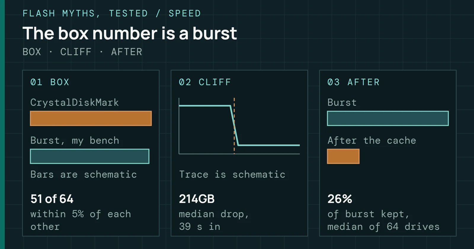
The throughput number on the spec sheet is real. It was measured under conditions that rarely match your workload, your fill level, or a drive after months of continuous writes.
Flash Foundations
Flash Foundations, Part 9: Performance & Endurance
Connect workload, write amplification, and cell wear to real drive behavior.
On this page 23 sections
Part 8 completed the stack with error correction. This part covers the performance and endurance figures on a spec sheet. They are what the whole stack adds up to. It also covers how vendors derive them and when a real drive matches them.
Why does one drive post a high number in a short test and a far lower one after hours of writing? Why do two drives with the same rating wear out at different rates? A short list of mechanisms answers both. The list is overprovisioningOverprovisioning is flash capacity held back from the user. The controller uses it as working space for garbage collection, which lowers write amplification. (OP), caching in single-level cell (SLC)The SLC cache may shrink as the drive fills. Writes run fast until it is full, then fall to the speed of direct TLC or QLC writes. mode, steady state, tail latency, and the write amplification behind terabytes written (TBW)Terabytes written is the total host data a manufacturer rates a drive to absorb over its life under the warranty conditions. and drive writes per day (DWPD)Drive writes per day is the number of times the full capacity can be written each day for the warranty period, which equals TBW divided by capacity and days. ratings. By the end you can read a spec sheet for its assumed conditions and treat a performance drop as a clue to its cause.
Overprovisioning: the capacity you cannot see
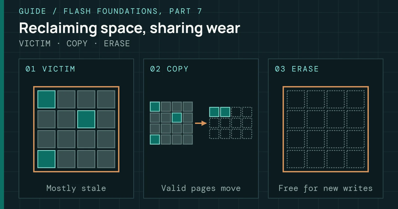
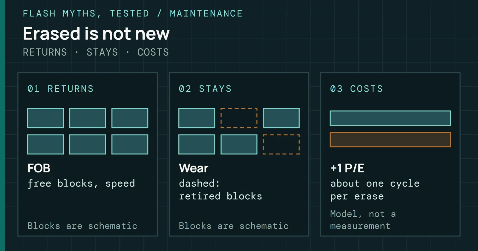
Every SSD reserves part of its raw NAND for internal use, and none of that space appears to the host. It does three jobs. First, it gives garbage collectionGarbage collection copies the valid pages out of mostly stale blocks and erases those blocks, so there is always free space for new writes. (GC) room to work without competing with incoming writes (Part 7 covers GC). More free blocks let GC choose better victim blocks and keep the write queue from backing up. Second, it lets worn blocks retire early, because spare blocks can replace them. Third, it replaces bad blocks, which NAND arrives with and develops over its life.
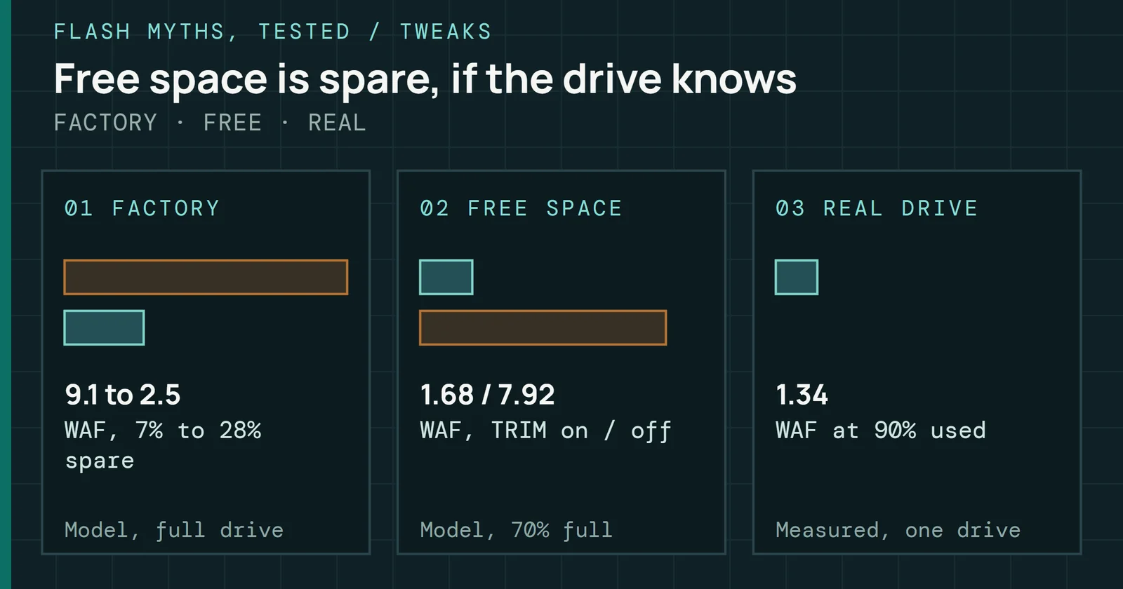
NAND is sized in GiB (1,024³ bytes) and drives are sold in GB (1,000³ bytes). Take a drive with 1,024GiB of raw NAND. It holds about 7.37% more than 1,024GB, and that gap is spare space on every driveInherent overprovisioning comes from raw capacity counted in binary units against a decimal user capacity, and it gives about 7.37% extra space.. Measured against raw NAND instead of the 1,024GB, the same gap is 6.9% of the total. Vendors quote OP as reserved capacity measured against user capacity, and they quote it on top of that gap, so total OP runs higher than the label.
Overprovisioning: the capacity you cannot see
Part of every drive’s raw NAND is never shown to the host
Raw NAND as 100%, two marketed OP levels
Figure 9.1 splits raw NAND into three parts at two marketed OP levels, as shares of the raw total. In both bars the GiB-to-GB gap is the same 6.9% slice. Copper marks what the vendor adds. It comes to about 6% of raw NAND at 7% marketed OP and about 20% at 28%, and total OP rises alongside. Seagate’s own table pairs a marketed 7% with a true physical OP of 15%, and a marketed 28% with 37%.
Seagate puts the manufacturer default for consumer drives at around 7 to 10% and suggests 20 to 28% for professional and enterprise drives in high-write use. A research paper on write amplification sets 0.28 as the factor used in commercial enterprise SSDs.
| Drive class | Marketed OP | What the vendor optimizes |
|---|---|---|
| Consumer | 7–10% | Usable capacity per dollar |
| Professional and write-heavy | 20–28% | Heavier mixed workloads |
| Enterprise | 28% | Consistent latency and life under sustained writes |
At 7%, a drive maximizes usable capacity per dollar, which suits price-sensitive consumers who rarely sustain heavy writes. At 28%, a drive gives up about a fifth of raw capacity. In return it buys consistent latency under sustained writes, lower write amplification factorWrite amplification factor is the data written to NAND divided by the data the host wrote. A value of 1 means no extra internal writes. (WAF) and longer life. Part 7 defines WAF and plots how steeply it falls as OP grows.
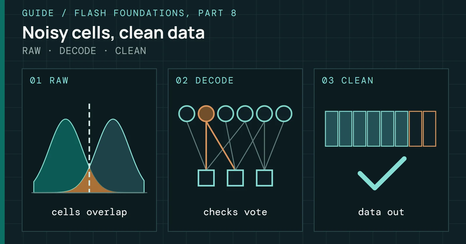
Error correction draws on the same raw space. Parity bytes sit in the NAND too, so a stronger code (one with a lower code rate) leaves less of the array for OP. A survey of flash errors works the case of a drive sold as 2.0TB with 2.4TB of physical NAND. That is a 20% surplus. At rate 0.93 a code spends 7% of the physical space on parity and leaves 2.4 × 0.93 = 2.232TB for data, which is 11.6% above 2.0TB. At rate 0.90 it leaves 2.16TB, which is 8.0% above. Designers must choose how to split the surplus between parity and OP.
Proposed multi-rate designs start a new drive on a weak code with a small codeword, return the saved space to OP, and step up to stronger codes as the raw error rate climbs (Part 8 covers the codes). In that survey’s model, four codes at rates 0.90, 0.88, 0.86 and 0.84 outlast a fixed 0.84 code by 31.2% at 15% OP.
Some vendor tools set OP directly. On any drive, leaving part of a freshly erased drive unpartitioned does the same thing, as long as those logical block addresses are never written. That technique improves sustained write performance on consumer drives at the cost of addressable capacity, and how much it helps depends on how random the writes are. Leave a Quarter to Half of the Drive Empty works through the numbers.
SLC cache: why burst numbers look impressive
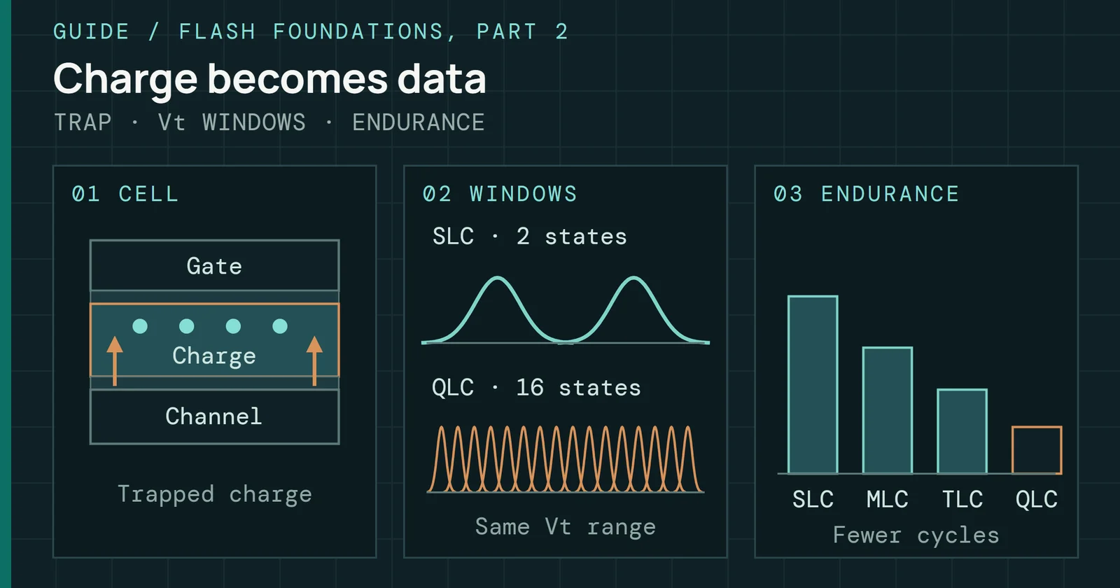
SLC caching exists because cell types differ in speed. A page programmed as SLC, with one bit per cell, needs only two voltage levels and typically programs in about 220µs on a classic 2Gb SLC part in Micron’s NAND technical note. The gap shows inside one modern part too. Frontgrade’s 4Tb triple-level cell (TLC) NAND data sheet lists a typical SLC-mode page program time of 226µs and a typical effective 1,900µs per page in TLC mode, about 8.4 times longer. Quad-level cell (QLC) dies are in the same range as TLC, and Intel’s 144-tier 1Tb die reported 1,630µs at ISSCC 2021, against 2,080µs for its 96-tier predecessor. Part 3 covers these timing parameters.
TLC and QLC drives use that speed. They write incoming host data to part of the NAND in SLC mode first, then move it to its permanent TLC or QLC location in the background. Part 6 covers the mechanism and the extra write it costs. This part covers the behavior the host sees.
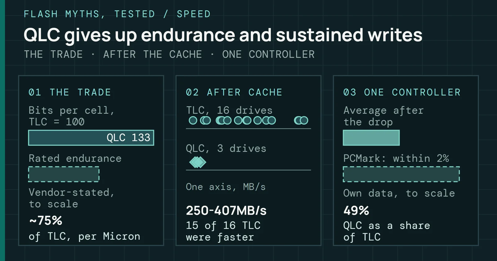
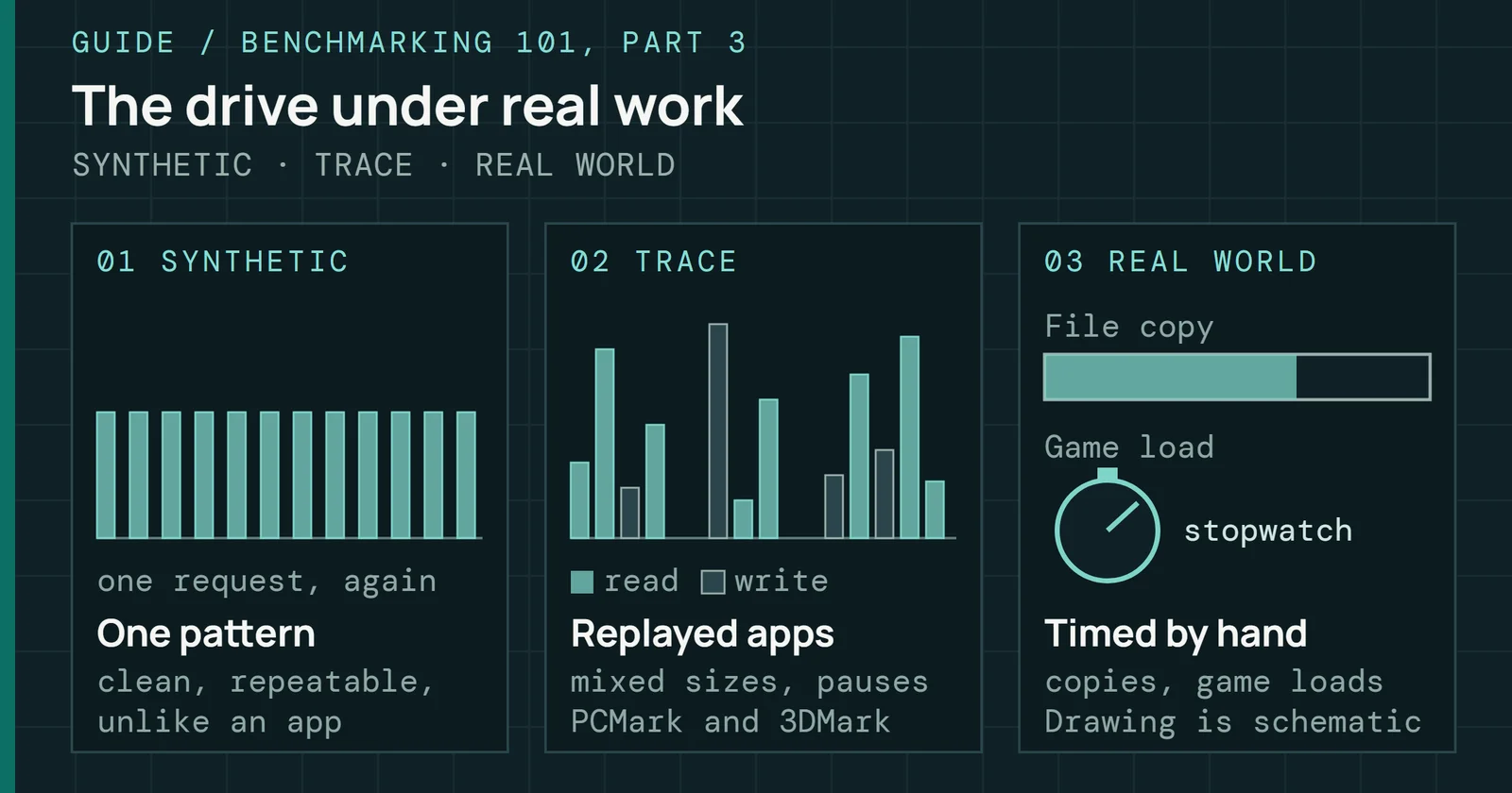
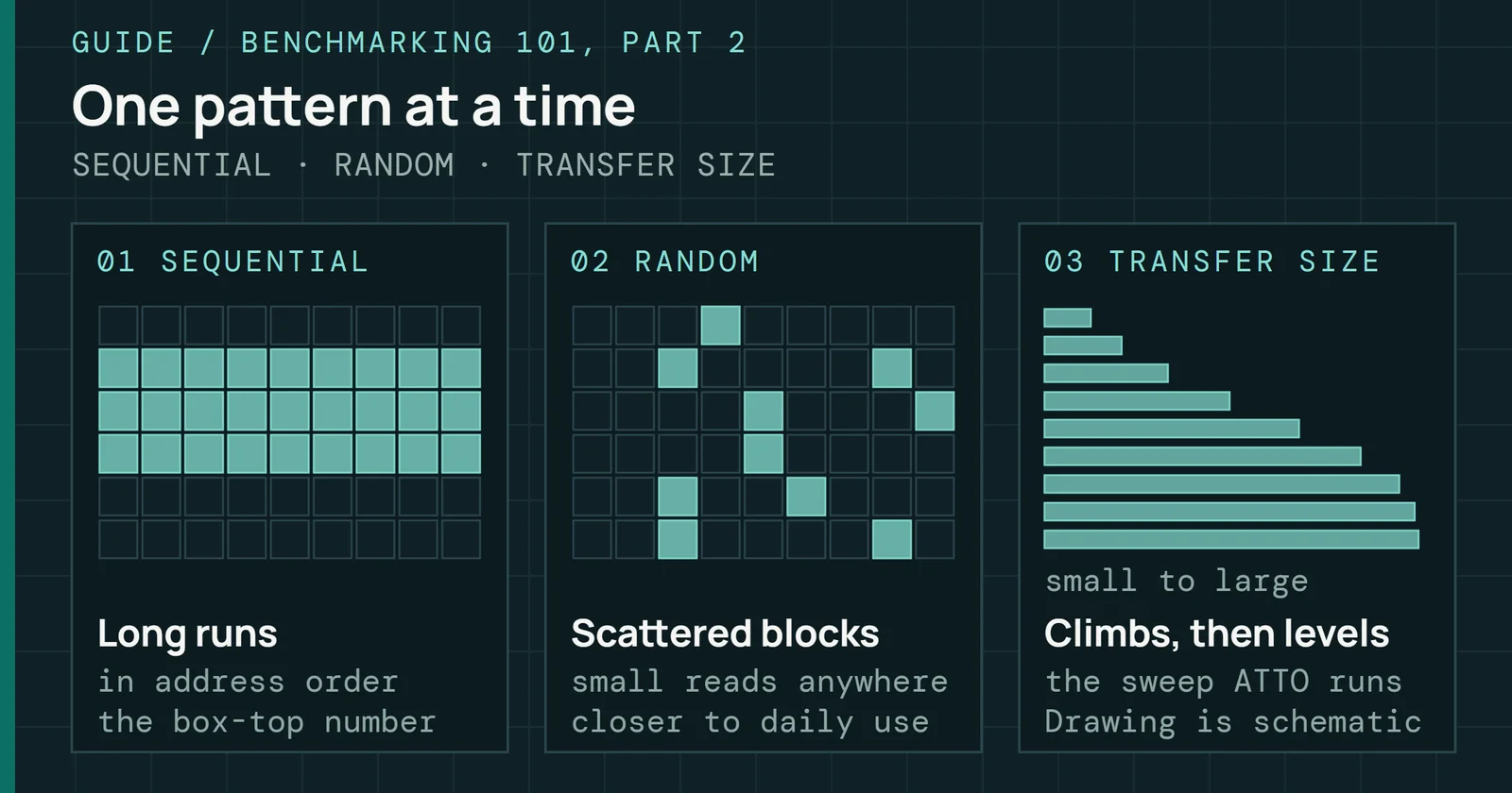
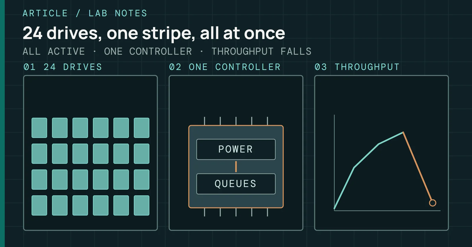
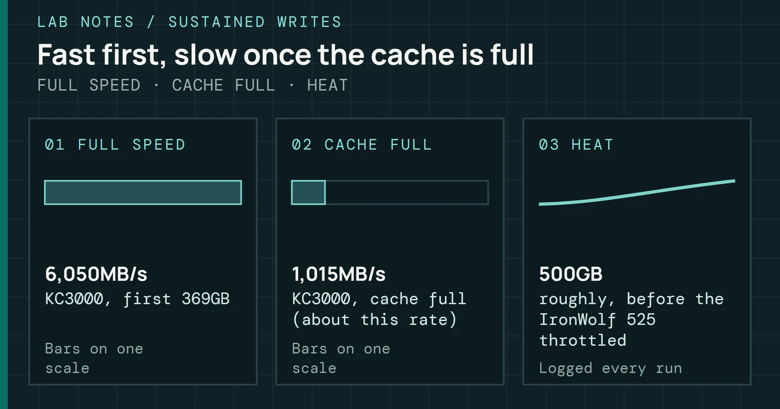
My own long sustained-write tests show the pattern. They used Iometer 1.1.0 on four drives, one run per drive, writing sequentially in 1MiB transfers at queue depth 32 and logging each second, for about 36 to 76 minutes per run. A TLC drive read near 6,000MB/s in its first seconds and held near 2,200MB/s late in the run. Three QLC drives started between about 2,900MB/s and 4,400MB/s and settled at 96 to 238MB/s. While the controller catches up on folding, the drive juggles incoming data, folding and GC at once, so firmware quality shows most in this window.
SLC cache: why burst numbers look impressive
Writes hold cache speed, then drop to native speed
Continuous sequential writes to one consumer NVMe drive
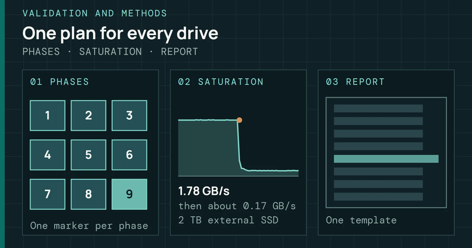
Figure 9.2 shows the drop in one drive’s own test log. Throughput holds near 4,400MB/s for the first 540GB written. Over the next 20GB bin the average is about 460MB/s, a blend of cache speed and native speed because the drop falls inside it. After that the line reads about 170MB/s and stays there for as far as the chart runs. That 170MB/s is a mean. The log runs on to about 1,275GB, and in its last third about 94% of the one-second samples sit near 96MB/s while about 5% are single-second bursts of up to about 1,900MB/s that lift the average to about 164MB/s. The median is 96MB/s, which is the figure Figure 9.5 uses for this drive. Here the cache is the share of the NAND that the firmware reserves as fast landing space, and writes past it run at native speed, so a long transfer sees the lower number.
Cache design varies by product class. A static cache has a fixed size, so it behaves the same at any fill level. Some drives skip the SLC cache and write straight to TLC. Solid State Storage Technology Corporation (SSSTC) pitches the same no-cache design for industrial and embedded systems that log data continuously. For them, predictable sustained write speed is the goal. Dynamic caches use empty TLC or QLC blocks as temporary SLC, which makes them large on a fresh drive and smaller as the drive fills. Hybrid designs combine a static minimum with dynamic expansion. Cache design is a firmware policy that stays invisible in the product listing and shows up clearly in sustained write tests.
Fill level and cache collapse: how a full drive behaves differently
Dynamic caching depends on free space. On a fresh or lightly filled drive, a large share of the free TLC blocks can serve as SLC for temporary write staging, up to a firmware-set cap. As the drive fills, those blocks hold permanent TLC data and are no longer available as SLC. Because most SLC cache designs size the cache from the data stored, the cache shrinks as the drive fills, and write behavior changes sharply.
Fill level and cache collapse: how a full drive behaves differently
Dynamic caches shrink as the drive fills, and static ones do not
Cache size as a share of the empty-drive dynamic cache
Figure 9.3 plots cache size against fill level for the three designs, with illustrative values. The dynamic line models a design that caches across all free space, so it falls in step with free space. About half is gone at 50% fill, and under a third is left at 70%. Static caches stay flat, and hybrids keep a static floor and add dynamic space above it.
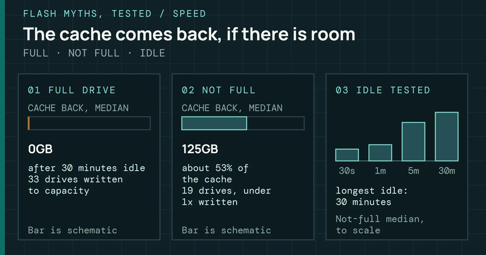
Nearly full dynamic-cache drives have almost no expandable SLC left. They run from a small fixed reserve, or straight from the free block pool with no cache at all, and the cliff in Figure 9.2 then arrives almost at once. Burst speed on a product page needs empty blocks, and a nearly full drive has few. Idle time doesn’t fix that. In my idle tests, most full drives got none of their cache back at speed after 30 minutes of rest, and Once the Cache Fills, the Drive Stays Slow has the data.
Another table walks the same trend by fill band. These are typical behaviors of dynamic-cache consumer drives, and no single drive was measured.
| How full | Dynamic SLC cache behavior | Write speed expectation |
|---|---|---|
| Mostly empty | Most of the SLC region available | Cache speed for most consumer workloads |
| Filling | Cache shrinking, GC recovery cycles visible on sustained writes | Cache speed with growing GC interruption |
| Mostly full | Minimal SLC headroom, GC competing with writes continuously | Sustained speed approaches native TLC or QLC, bursts shorter |
| Nearly full | Effective SLC exhaustion on dynamic-cache designs | Native TLC or QLC speed, GC latency spikes become frequent |
| Completely full | Controller in continuous emergency reclamation | Severely degraded throughput, unpredictable latency |
Drives that skip the SLC cache tolerate high fill levels far better. They write directly to TLC, so there is no cache to shrink and no cache cliffThe cache cliff is the sudden drop in write speed when the SLC cache is full. A fuller drive has a smaller cache, so the cliff comes sooner.. Random-write speed still falls as the drive fills, because free space acts as extra OP, and the larger OP on an enterprise drive keeps that fall shallow. Higher OP allocation gives GC more spare blocks at any fill level, which lowers WAF and keeps throughput steadier across a wider operating range.
Defining steady-state performance
Fresh-drive performance makes a poor specification for a deployed device. Drives reach steady stateSteady state is the condition where performance has stopped changing because the drive is full of data and garbage collection runs continuously. when enough write traffic has displaced its fresh-state advantage. At that point any SLC cache is either exhausted or cycling continuously, and GC runs at a rate matched to the incoming writes. Performance settles at a level the drive can hold for a long time under that workload. How long the drive takes to get there depends on its capacity and OP. Larger drives with more spare room need more data written before the fresh-state advantage is gone, which is why short tests of large drives mislead most.
The SNIA Solid State Storage Performance Test Specification (PTS) turns that idea into a test. It defines the purge, the workload-independent and workload-dependent preconditioning, and the steady-state measurement window. Results come only from that window. In PTS Enterprise 1.1 a tracked variable counts as steady when, across a five-round window, its range stays within 20% of its average and the slope of its best linear fit stays within 10% of that average.
Defining steady-state performance
Steady state starts when the curve stays inside a flat window
One-minute mean write speed, one TLC drive, long sequential run
Figure 9.4 applies that test to the log of the TLC drive’s run described above, which lasted about 75 minutes. Throughput reads near 6,000MB/s for the first seconds, so the first one-minute round averages 3,626MB/s. It drops as the cache empties, stays near 1,740MB/s through minute 15, then steps up and settles near 2,200MB/s. The copper rectangle is the last five one-minute rounds, a window where the rounds average 2,187MB/s, vary by 3.5% of that average and show a trend of 0.2%, well inside the PTS limits of 20% and 10%. My run isn’t a PTS run, because it has no purge or preconditioning and writes sequentially, so the figure shows how the window test reads a real curve. Any run that stops earlier reports a number the drive can’t hold.
Steady-state performance depends on free space, on how well GC keeps pace with the incoming write rate, on thermal state, and on workload pattern. Sequential workloads are easier on GC than random ones, because data written together tends to be overwritten together and so victim blocks hold few valid pages to copy. Mixed read and write traffic hurts read latency, because reads can queue behind program, erase, and GC copy operations on the same die.
Burst and sustained numbers: what the spec sheet cannot tell you
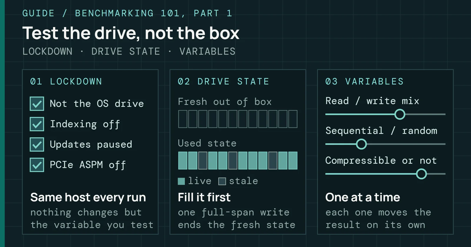
Spec sheets and quick benchmarks measure burst performanceBurst performance is what a drive does in the first seconds, helped by caches. Sustained performance is what it holds once those are used up. on an empty drive with a fresh format and a few seconds of sequential writes. Those conditions give the firmware every advantage. The SLC cache has room, GC has little to do, and channel parallelism is at its maximum. Such numbers look good but say almost nothing about real use.
Sustained testing fills the drive to a high occupancy, forces the controller into steady-state GC, and measures under continuous load. It shows real write speed after the SLC cache runs out, how well GC keeps free blocks available, and how steady latency stays under pressure. Users feel exactly these during large transfers or write-heavy production work.
The runs described above show how far apart two spec sheets can sit. Two of the QLC drives began at different speeds and landed on the same 96MB/s, and the TLC drive finished far above both. The difference reflects NAND type, die count, firmware quality, and OP allocation.
Burst and sustained numbers: what the spec sheet cannot tell you
A fast start says little about the speed late in the run
Four drives, one long sequential-write run each
Figure 9.5 puts the four drives side by side, with each drive’s first seconds against the median of the last third of its run. A fresh-state score tells you little about the late number. OP is one lever behind the difference. SNIA’s endurance white paper says write amplification falls as OP rises, so a drive with more spare NAND has to do less garbage collection work per host write. The design envelope shows up only at steady state.
Validation-grade sustained testing adds stressors that a single steady-state run misses. Three common ones follow.
Queue depth transitions
The test cycles the queue depth across its range during a write run, which stresses the controller’s arbitration and scheduling.
Read-disturb injection
The test interleaves heavy reads of addresses in the blocks the write workload is filling, which disturbs the unread wordlines in the same block and shifts their threshold voltages.
Thermal stress
The test holds the workload while the controller approaches its junction temperature limit, so throttling and its recovery show up in the latency trace.
Latency percentiles: the metrics that matter
Peak throughput captures headlines. Latency percentiles determine the experience. Even a drive that delivers 5,000MB/s of peak sequential throughput can still deliver a poor experience if its latency distribution is wide. Interactive and production workloads care about the tail more than the best case, and the questions are how often the drive responds much slower than usual, and by how much.
Scale makes the tail visible to everyone. Dean and Barroso measured a large fan-out service whose 99th-percentile latency for a single random request to finish was 10ms, but 140ms for all the requests to finish.
The standard percentile framework in storage engineering:
- p50 (the median): 50% of operations complete within this latency.
- p99: 99% complete within this latency.
- p99.9: 99.9% complete within this latency.
- p99.99: 99.99% complete within this latency.
Because no standard fixes the ranges, the table gives illustrative figures by drive class for 4KB reads at queue depthIOPS counts commands finished per second. Queue depth is how many commands are outstanding at once, and a drive needs a deeper queue to reach its top IOPS. 1 (QD1) and for mixed load. Part 1 covers queues. Treat them as rules of thumb. An enterprise drive that publishes a quality-of-service figure, usually p99.9 and beyond, is the better source for that drive. Micron’s 7450 data sheet is one example. At SNIA PTS steady state and queue depth 1 it lists a median read of 80µs and a 99th-percentile read of 90 to 95µs, with 15µs and 65µs for writes.
| Drive class | Typical p50 (4KB read, QD1) | Typical p99 (mixed load) | Typical p99.9 (mixed load) | Primary p99.9 driver |
|---|---|---|---|---|
| Consumer SATA | 80–100µs | 200–500µs | 2–10ms | GC interruptions, and TRIM on drives without queued TRIM stalling the Native Command Queuing (NCQ) queue |
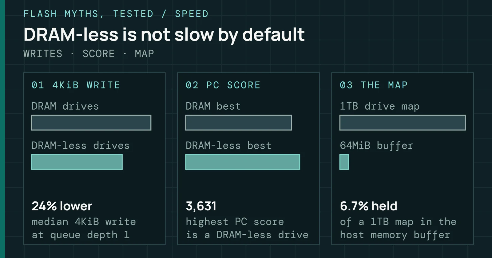
| Consumer NVMe, DRAMless | 40–70µs | 200–800µs | 5–30ms | Logical-to-physical (L2P) map lookup on NAND, GC combined with cold-map reads |
| Consumer NVMe, DRAM-backed | 30–60µs | 100–300µs | 500µs–3ms | GC interruptions, SLC cache exhaustion under burst write |
| Enterprise read-intensive | 50–80µs | 150–400µs | 300µs–1ms | Infrequent GC, tR (page read time) variation with wear |
| Enterprise mixed-use (3 DWPD) | 60–100µs | 200–600µs | 0.6–1.5ms | Sustained GC pressure, write amplification under mixed load |
Ranges reflect steady-state performance on warmed drives at typical occupancy, 50 to 70%. Tail latency widens as the program/erase (P/E) cycle count approaches end of life, because of read retry latency and longer tBERS (block erase time) from oxide-degraded blocks.
Latency percentiles: the metrics that matter
The tail is far wider than the median, and it differs by drive class
p50 for 4KB reads at QD1, p99 and p99.9 under mixed load, three of the five classes
Figure 9.6 plots the geometric midpoint of each table range (the square root of the low end times the high end) on a log axis, with the range itself drawn as a thin bar behind each dot. All three classes sit within a factor of two of each other at p50. The median hides a gap that shows at p99.9. There the DRAMless midpoint is about 12ms, which is about ten times the DRAM-backed midpoint of about 1.2ms and about thirteen times the enterprise mixed-use midpoint of about 0.9ms.
GC effects begin to show at p99 and dominate the p99.99 outliers, and long block erases are a known source of read tail latency. Once the controller must reclaim blocks before it accepts a new write, that command’s latency spikes. At 10,000 input/output operations per second (IOPS), p99.99 is one slow command per second. If each of those commands stalls for 100ms, a latency-sensitive application stutters once a second. Wear widens the tail on its own, even without GC pressure. As P/E cycles pile up, erases take longer and reads need more retry steps, so a growing fraction of commands run long. Part 3 covers the physical mechanism.
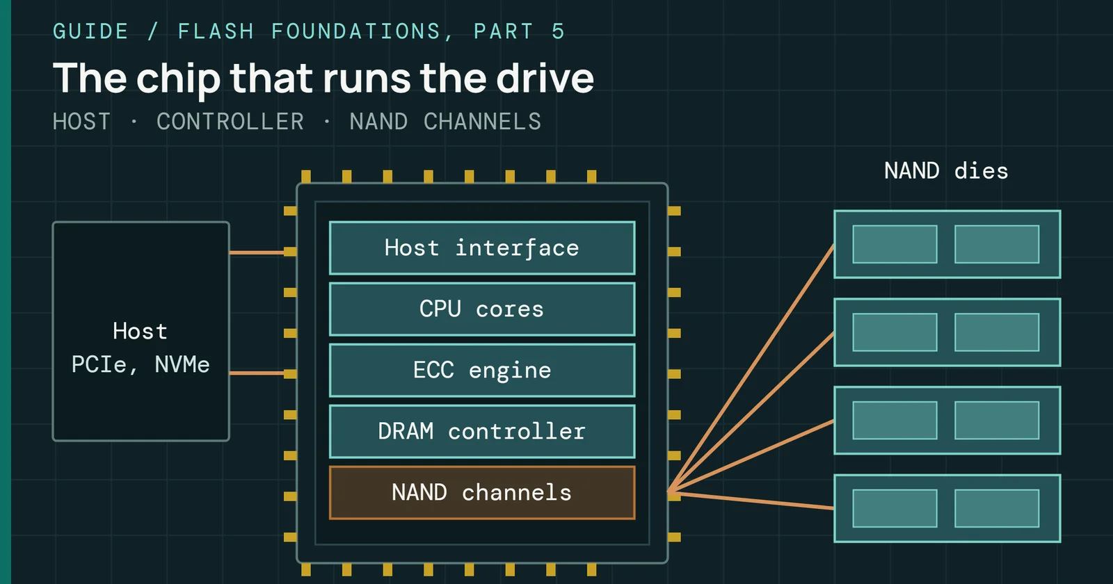
Enterprise SSDs prioritize latency consistency over peak throughput. Higher OP provides more free blocks and fewer GC interruptions, and predictive GC reclaims blocks before the free pool runs out. Power-loss protectionPower loss protection uses stored energy to let a drive finish writing buffered data and metadata when power fails, so acknowledged writes survive. (PLP) lets firmware treat its DRAM write buffer as safe (Part 6 covers PLP), so the capacitors finish in-flight work on power loss and the drive skips conservative flushes that stall commands. Together these give tighter tail latency at the cost of slightly lower peak throughput, which suits latency-sensitive production deployments.
Endurance ratings: what they assume and what they do not say
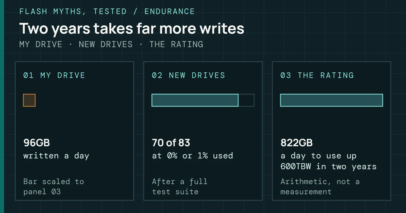
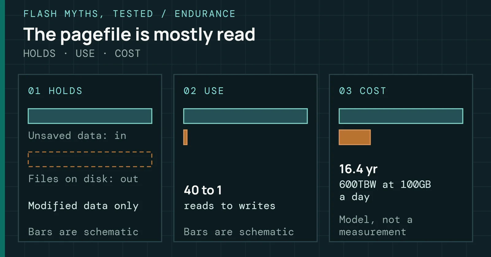
SSD endurance is rated in TBW or DWPD, and both state how much the drive is warranted to write before the manufacturer’s coverage ends. A 1TB drive rated at 600TBW can sustain 600 terabytes of host writes over its warranty period, and the 870 EVO data sheet carries the same 600TBW for its 1TB model. At 100GB a day, reaching 600TBW would take about 16 years, so a typical five-year warranty runs out first. For a write-heavier case, take a 1TB enterprise drive rated at 3 DWPD for five years (Kioxia offers enterprise models at 3 and 1 DWPD). It can sustain 3 terabytes written per day, about 5,475TBW in total.
How a rating is built
Both ratings are one budget in two forms. TBW and DWPD ratings are calculated from the NAND’s P/E cycle budget, OP allocation and an assumed WAF. Divide TBW by the drive capacity and the warranty days to get DWPD.
Endurance ratings: what they assume and what they do not say
A rating is a wear budget divided by an assumed WAF
Four steps from NAND wear to DWPD
Figure 9.7 follows the budget through four steps. Roughly, TBW is the NAND capacity times the rated P/E cycles, divided by the total WAF the rating assumes. Ratings are accurate under their assumptions. Deployments whose real WAF differs deliver a different effective TBW, and Part 7 works through that case. Divide TBW by the host’s daily writes to get years of life.
That same budget gives years of life directly. The survey of flash errors states the model manufacturers use:
Years of life = PEC × (1 + OP) ÷ (365 × DWPD × WAF × R_compress)
PEC is the P/E cycle endurance of each block. OP is the total spare space (the physical capacity minus the user capacity, divided by the user capacity), so it includes the GiB gap. PEC × (1 + OP) is then the number of full drive writes the drive can absorb. DWPD is the workload’s daily full-drive writes, WAF is the write amplification factor, and R_compress is the compressed size divided by the original size. Controllers with no compression set R_compress to 1. As an illustration, say a drive has 3,000 cycles per block, 7% total OP, a WAF of 3 and a host that writes half the drive each day. It lasts 3,000 × 1.07 ÷ (365 × 0.5 × 3) = 5.9 years. If the data compresses to half its size, R_compress is 0.5 and the same drive lasts 11.7 years, because it programs half as much NAND per host write.
The workload sets DWPD and R_compress. Compression only helps when the data is compressible, and work on compression inside the SSD found that, on an emulated SSD running a database workload, compressing in the drive’s firmware beat compression in the file system or the database, and cut the data written to flash and the garbage collection overhead. Already-compressed data such as video leaves R_compress at 1.
What a rating requires
JEDEC JESD218 sets the endurance method, and under it a rating stays valid only if the drive still meets four conditions at that many terabytes. The drive keeps its capacity, it holds the uncorrectable-error target, it stays within the functional failure limit, and it retains unpowered data for the required time. Client and enterprise classes set different bars. Part 8 covers the error targets and the retention targets.
The functional failure limit is 3% or fewer, set at 60% statistical confidence, and the confidence level drives the sample size. Take a Poisson upper bound on the failure rate. It is one common way to compute the limit, a calculation of my own rather than a table from the standard. Zero failures in N drives supports a rate of at most about 0.92 ÷ N at 60% confidence, so showing a 3% limit takes about 31 drives. Allowing one failure raises that to about 68 drives, and two failures to about 104.
What fleets show
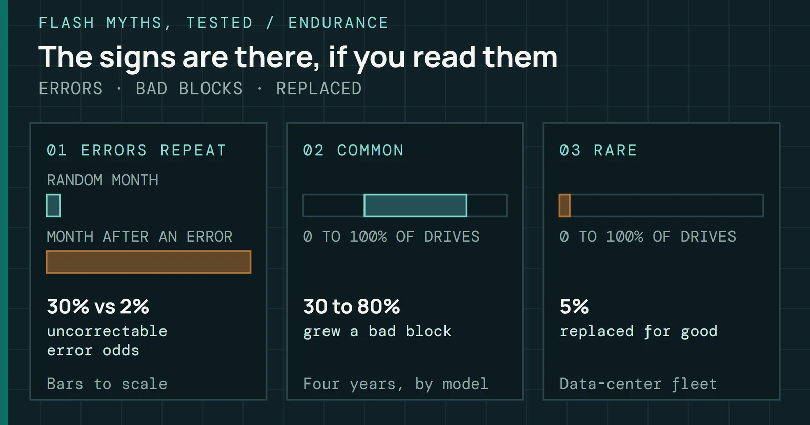
Ratings describe a population, and the field is lumpier. A study of flash failures in Facebook’s data centers followed several drive platforms for nearly four years. It counted a drive as failed once it reported at least one uncorrectable error, and between 4.2% and 34.1% of the drives in a platform had. Within every platform, the 10% of drives with the most errors held over 80% of that platform’s uncorrectable errors. In four of the six platforms, the top 10% held over 95%. Errors also repeat. Across one recent two-week window, 99.8% of the drives that had an error in the first week had one in the second.
Failure rate did not simply grow with the data written to a drive. It rose in an early detection period, fell in an early failure period as the controller retired the weakest blocks, and rose again through the useful life and wear-out. The authors propose a weak pool of blocks that fails and is retired early and a strong pool that lasts. Early detection ended at about 3TB written on the 720GB and 1.2TB drives and at about 10TB on the 3.2TB drives. TBW ratings say nothing about where on that curve one drive sits.
Sanitizing spends the budget
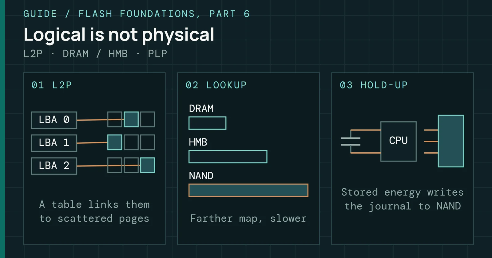
Part 6 covers the sanitize variants and what each costs. Block Erase Sanitize erases every writable block, which by simple counting spends about one P/E cycle per block and up to about one full drive write of budget. That is trivial on a healthy drive and matters near end of life, where a failed sanitize leaves the media partly wiped and the security requirement unmet. Crypto Erase replaces the media encryption keys and by default spends no P/E cycles. Fleets that sanitize at end of lease should count one sanitize event in the endurance they buy.
DWPD tiers: matching a rating to a workload
DWPD follows from the cell type’s P/E budget at its rated retention class, OP allocation, the WAF the rating assumes, and the warranty period, so it is a design outcome and no fixed property of the NAND. Tiers on sale reflect different customers with different write rates.
DWPD tiers: matching a rating to a workload
TBW grows in a straight line with DWPD
1TB drive, five-year warranty
Figure 9.8 shows what a tier means in terabytes for one 1TB drive over a five-year warranty. TBW grows in a straight line with DWPD, so a 3 DWPD drive is built to spend about seven times the write budget of a 0.42 DWPD drive. Part 2 gives the cell physics behind those budgets.
The table lists published ratings from each tier, with the cell type, an example drive, and the workload the maker or SNIA pairs with it. SNIA calls 1 DWPD typical for mainstream read-intensive enterprise drives and 3 DWPD the mixed-use class for caching, database and higher-write work.
| DWPD rating | Cell type | Example drive | Target workload |
|---|---|---|---|
| 0.42–0.60 | QLC | Solidigm D5-P5336, 7.68TB to 122.88TB | Read-dominant archive, cold storage, CDN caching |
| 1 | TLC | Micron 7450 PRO | Read-intensive and mainstream enterprise |
| 3 | TLC | Micron 7450 MAX | Mixed-use enterprise, caching, databases |
| Up to 50 | SLC | Solidigm D7-P5810 | Write-intensive, logs and caching |
Tiers differ in write budget per day. A 1TB drive rated at 0.42 DWPD is budgeted for 767TBW over five years, against 5,475TBW at 3 DWPD (Figure 9.8), so a workload that writes more per day than a drive’s rating assumes spends the warranty budget early. Compare the rating with the workload’s actual write rate.
Spare capacity is one lever behind a higher rating. The drive sells fewer of its raw gigabytes, and the DWPD calculation above shows why that helps. PLP and the controller are separate choices that shape latency and power-loss behavior, and the rating itself follows the P/E budget, OP and assumed WAF.
Thermal throttling: thresholds, hysteresis and the power cap
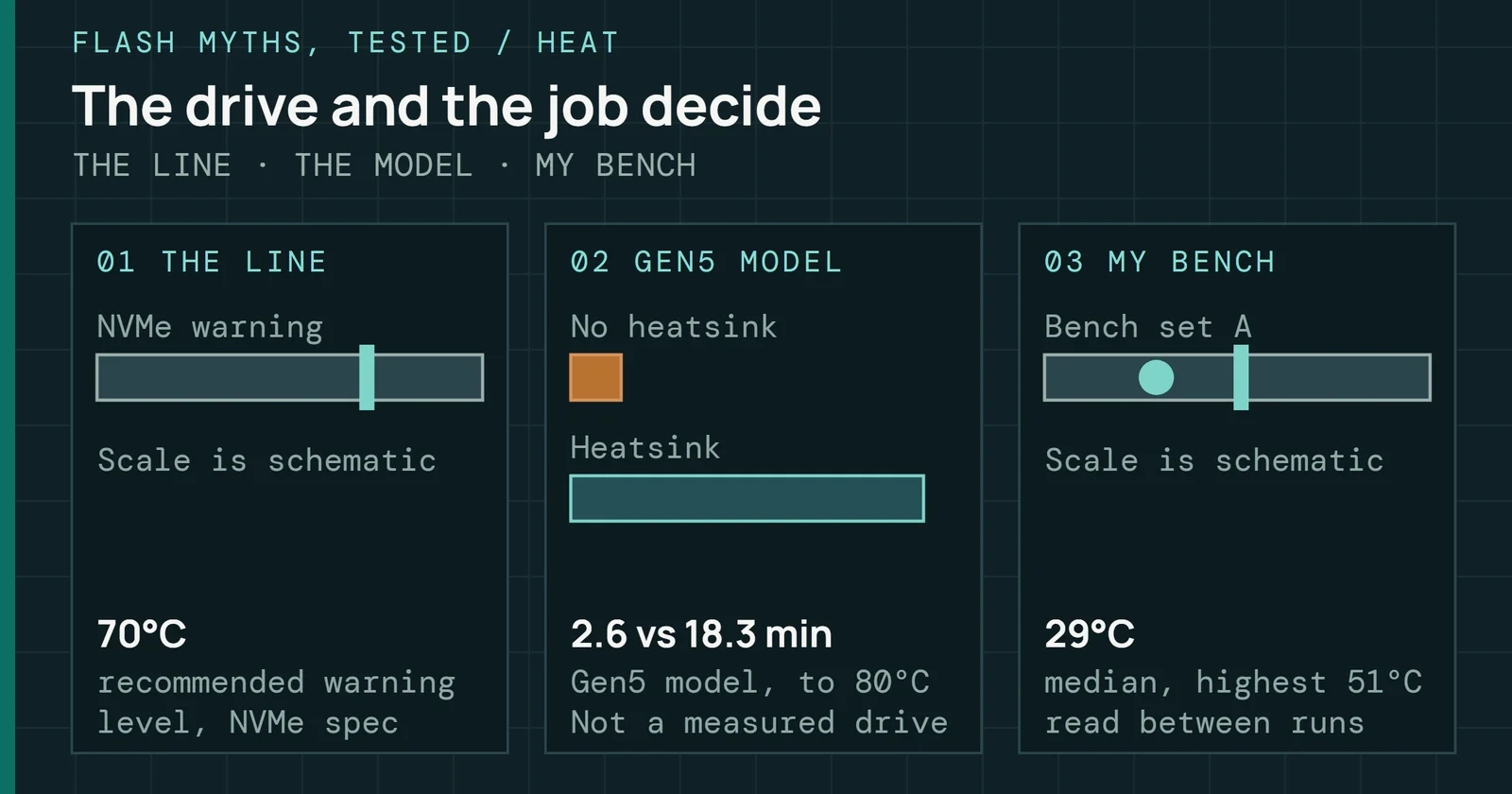
NVMe defines two temperature thresholds in the Identify Controller data. They are WCTEMPWCTEMP is the warning temperature and CCTEMP the critical one. TMT1 and TMT2 are host-set points at which the drive starts to throttle. (Warning Composite Temperature Threshold) and CCTEMP (Critical Composite Temperature Threshold). The Self-Monitoring, Analysis and Reporting Technology (SMART) / Health Information log reports the Composite Temperature and the minutes spent above each. WCTEMP marks overheating where operation continues but remediation is recommended. CCTEMP marks a critical condition that can force throttling, shutdown, or data loss. Temperatures arrive in kelvins, and the spec only recommends that a drive report 0157h for WCTEMP, which is 343K or about 70°C. Vendors set both thresholds and they differ by model, so read them from the drive instead of assuming a value.
Thermal throttling: thresholds, hysteresis and the power cap
A throttled drive recovers only after cooling well below trip
Three thermal states of an NVMe drive
Figure 9.9 shows the three states. Where throttling starts is the vendor’s choice, and it can sit at or below WCTEMP. Throttling lowers throughput by doing less NAND work per unit of time and leaves array timings such as read time (tR), program time (tPROG), and block erase time (tBERS) alone. Controllers differ in how they do it. Some step through a table of speed levels, some wait between commands, and some lower the PCIe link rate. Hosts see lower sustained throughput but no I/O errors, since throttling is a protection response and counts as no failure mode.
Recovery takes time. Controllers commonly use a hysteresis band, and the drive stays throttled until temperature falls well below the trigger point, which prevents oscillation at the margin. If the thermal environment is borderline, a drive that enters throttle may stay throttled longer than the momentary spike suggests. At CCTEMP, behavior varies. Some controllers halt non-critical activity and others force a controlled shutdown. Sustained operation near CCTEMP calls for a thermal fix, because firmware tuning cannot cure its environment.
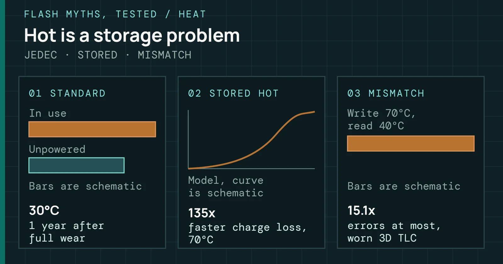
Field data shows the same split between heat and the response to it. In the fleet study, failure rates in the study’s figures between 30°C and 40°C held level or rose slightly with temperature. Above 40°C the trend depended on the platform. Failure rates rose with temperature on two platforms, were less sensitive on two, and fell on the last two. Those two least sensitive platforms throttled most aggressively, and the authors conclude throttling appears to greatly reduce the reliability cost of higher temperatures. Hot NAND Is Bad for Your Data works through that study, and Every NVMe SSD Needs a Heatsink covers what cooling changes in practice.
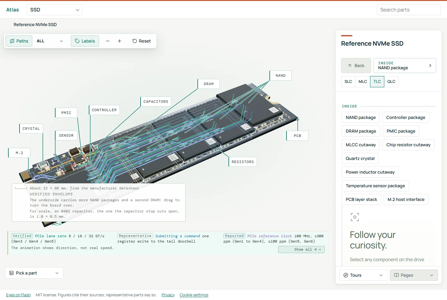
Up to nine temperature values come from the NVMe log. One is a Composite Temperature and the rest are Temperature Sensors 1 through 8. The spec says the composite may not represent the actual temperature of any physical point, and sensor placement is up to the vendor. Some designs add a separate sensor on the board. TechInsights’ teardown of the Crucial T705 names a Texas Instruments TMP108 digital temperature sensor, and TI pitched its SSD PMIC alongside a temperature sensor such as the TMP121. When the composite and an individual sensor disagree under load, read the individual sensors before deciding where the heat is.
A power cap is a different lever
Thermal throttlesThermal throttling slows a drive when its temperature passes a limit, cutting power and heat so the hardware stays within its safe range. react to temperature, while a power cap limits how much current the NAND draws at once, whatever the temperature. Programs running on many dies at the same moment can draw more current than the drive’s power budget allows, which limits how much parallelism a design can use. One way to cap the peak is to suspend upper-page programs. They are the longest and most energy-hungry program step, and suspending them keeps peaks from different dies from stacking. Program suspendProgram and erase suspend let a die pause a long operation to serve a read, then resume, which cuts the wait that reads would otherwise see. is best known as a way to cut read latency, and it works as a power tool too, at the cost of longer program time. The Throttle Lab has a program suspend setting that shows the trade.
Unlike a thermal throttle, a power cap stretches program time while barely moving average power, so the heat barely moves either. Power caps can therefore show up as longer write latency while the temperature log stays flat. Telling the two apart takes the temperature log next to the latency trace. FlashPower is a published model for estimating NAND power per operation. Gen5 drives need heatsinks and airflow to hold up under sustained load.
In the field: reading a slow or worn drive
Any drive that performed well and now performs poorly has changed its internal state, and the decline is a symptom. Start with the cheap checks. The OS shows logical fill level directly, and SMART Data Units Written (counted in units of 512,000 bytes) divided by capacity shows how many full drive writes the drive has absorbed. Nearly full drives that benchmark far below spec are often operating as designed, because the spec conditions do not apply to it. When fill level and temperature leave the slowdown unexplained, the cause usually fits one of four patterns.
In the field: reading a slow or worn drive
Two log fields split a slow drive into four likely causes
Temperature first, then spare capacity
Figure 9.10 orders the checks by cost. Part 8 owns the SMART field reference, so this section names only the fields it uses, which are Available Spare, Percentage Used, Data Units Written, and Composite Temperature.
Effective OP exhaustion
As blocks retire from wear or defects, the free block pool shrinks. GC has less room, WAF climbs, and sustained write throughput drops. That drive still works but settles at a permanently lower level. The SMART Available Spare field shows the share of spare capacity that remains, so the decline is visible. Part 6 covers how retired blocks drain that reserve.
Elevated block retirement rate
Healthy drives retire blocks slowly and predictably. Higher-than-expected WAF, a workload mismatch, or marginal NAND from a low-yield lot makes blocks retire faster than the baseline predicts. Available Spare then falls faster than the observed write volume explains, and fleet telemetry catches it before the drive surfaces errors. Part 7 shows how to compute the rate.
Thermal throttling
NAND timing and controller behavior depend on temperature. Drives that were once thermally adequate but now run hot because of changed airflow or adjacent heat may stay throttled as long as the heat source remains. Check Composite Temperature against throughput.
Component substitution within a model
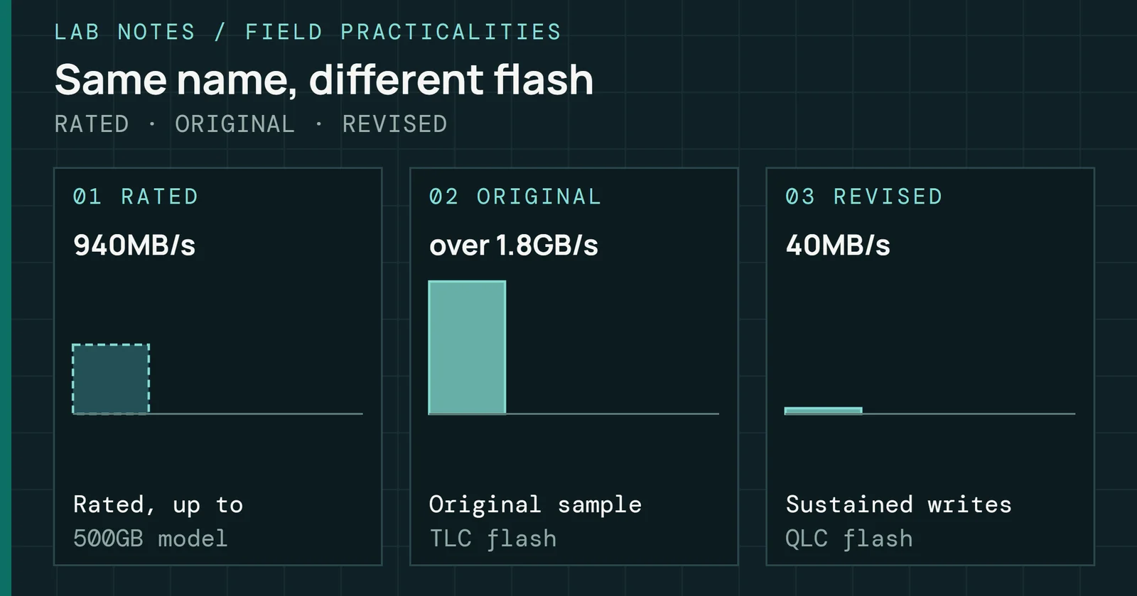
NAND type and vendor can change within one model number without any change to the listing. Samsung’s 970 EVO Plus, for example, changed from the Phoenix controller to Elpis under the same name. Fleets see it as a replenishment batch that benchmarks differently from the original batch at equal wear, or wears at a different rate under the same workload. The Field Practicalities covers a real case. The Crucial P2 went from TLC to QLC flash under the same name. In Tom’s Hardware’s review, sustained writes fell to 40MB/s after the cache filled.
The table pairs each symptom with its likely cause, the first metric to check, and a remediation to try before replacing the drive.
| Symptom | Root cause | Metric to check | Remediation |
|---|---|---|---|
| Sustained write throughput declining, no errors surfaced | Effective OP exhaustion from accumulated block retirement | Available Spare approaching its threshold, WAF above the workload baseline | Assess workload fit, consider a higher-OP drive |
| Spare capacity declining faster than write volume predicts | Accelerated retirement from workload mismatch or marginal NAND | Spare decline rate against Data Units Written, compared with the fleet cohort at the same wear | Investigate WAF, compare with the fleet baseline, escalate if an outlier |
| Slow only under sustained load, drive runs hot | Thermal throttling | Composite Temperature in the SMART / Health Information log, correlated with latency spikes | Improve chassis airflow, verify heatsink contact, find adjacent heat sources |
| Replenishment batch underperforms the fleet at equal wear | NAND substitution within the same model | Sustained write throughput after cache exhaustion, and wear rate per TB written, against the original batch | Re-qualify against the original baseline, check the NAND revision through a vendor log if available |
Throughput alone hides the tail. Across a fleet running one workload, watch for outliers. A drive with clearly higher p99.9 latency than its cohort over several days is worth pulling before it fails in front of a customer. That comparison needs a tool that records the latency distribution.
What performance and endurance hand to the future
Write amplification, wear, spare capacity and tail latency are the signals that the firmware in the next part acts on.
What performance and endurance hand to the future
Performance & Endurance feeds one later part.
Arrows run to the parts that build on this one.
Part 10 closes the series with what comes next. It covers firmware that watches wear, classifies workloads at runtime, and adapts GC, ECC thresholds and write policies on the fly. It also covers how machine learning, ZNS, CXL, and computational storage change what drives need from the host.
Sources
Primary is the original paper, standard or datasheet. Secondary is a review, a vendor summary or a news report. Measured is my own test data.
Show all 32 sources, 24 primary
- PrimaryMicron TN-29-19, NAND Flash 101 (Rev. B, 2010)Micron Technology, Inc., 2010
- PrimarySNIA Solid State Storage Performance Test Specification (tutorial)SNIA, 2011
- PrimarySolid State Storage (SSS) Performance Test Specification (PTS) EnterpriseSNIA, 2013
- PrimaryThe Tail at ScaleCommunications of the ACM, 2013
- PrimaryCompression and SSD: Where and How?INFLOW 2014 (USENIX workshop), 2014
- PrimaryA Large-Scale Study of Flash Memory Failures in the FieldACM SIGMETRICS 2015, 2015
- PrimaryRead Disturb Errors in MLC NAND Flash Memory: Characterization, Mitigation, and RecoveryCarnegie Mellon University SAFARI Technical Report 2015-006, 2015
- PrimaryError Characterization, Mitigation, and Recovery in Flash-Memory-Based Solid-State DrivesProceedings of the IEEE, 2017open copy
- PrimaryPractical Implication of Analytical Models for SSD Write AmplificationACM/SPEC ICPE 2017, 2017
- PrimaryIntroducing the Solidigm D7-P5810 – an ultra-fast SLC SSD for write-intensive workloadsSolidigm newsroom, 2023
- PrimaryNVM Express Base Specification, Revision 2.1NVM Express, Inc., 2024
- PrimaryMicron 7450 SSD Series Technical Product SpecificationMicron Technology, 2026
- PrimarySSD Product Warranty | SupportSamsung Semiconductor Global, 2026
- PrimaryDeep Dive Teardown of the Crucial T705 CT2000T705SSD5 SSD (TechInsights)TechInsights
- PrimaryEndurance of NVMe, SAS, and SATA SSDsSNIA
- PrimaryEnterprise SSDKIOXIA America, Inc.
- PrimaryFrontgrade UT81NDQ512G8T: 4Tb TLC NAND Flash datasheet
- PrimaryJEDEC SSD Specifications ExplainedJEDEC
- PrimaryJEDEC SSD Specifications Explained: JESD218 and JESD219 (Alvin Cox, Seagate)JEDEC
- PrimaryPractical Erase Suspension for Modern Low-latency SSDsusenix.org
- PrimarySamsung SSD 870 EVO Data Sheet, Revision 1.1Samsung Semiconductor
- PrimarySolidigm D5-P5336: product briefSolidigm
- PrimaryTI introduces industry's smallest power management ICs for solid state drives (TI.com)Texas Instruments
- PrimaryWhat Is SSD Over-Provisioning?Seagate
- SecondaryIn-place Switch: Reprogramming based SLC Cache Design for Hybrid 3D SSDsarXiv, 2024open copy
- SecondaryCrucial P2 M.2 NVMe SSD Review: Beating SATA Dollar for Dollar (page 2)Tom’s Hardware
- Secondarynvme_smart_log(2) — libnvme-dev — Debian testing — Debian Manpagesmanpages.debian.org
- SecondarySamsung is swapping parts in their 970 Evo Plus SSDs and sabotaging performance (TechSpot)TechSpot
- SecondarySATA 6Gb/s SSD Controller with NANDXtend™ TechnologyONFI
- SecondarySolidigm 122.88TB D5-P5336 Review: High-Capacity Storage Meets Operational EfficiencyStorageReview.com
- SecondaryWhat is Direct Write ? (SSSTC)SSSTC
- MeasuredThe author’s own measurements