Picture two drives with the same NAND, the same controller and the same firmware build. Three years in, one still delivers its rated write throughput. Its twin fell off a performance cliff early in its life. The difference is how hard garbage collectionGarbage collection copies the valid pages out of mostly stale blocks and erases those blocks, so there is always free space for new writes. (GC) had to work under each drive’s write load, overprovisioningOverprovisioning is flash capacity held back from the user. The controller uses it as working space for garbage collection, which lowers write amplification. (OP) and TRIMTRIM, called Deallocate in NVMe, tells the drive which logical blocks the file system no longer uses, so garbage collection need not copy them. configuration.
Flash Foundations
Flash Foundations, Part 7: Garbage Collection & Wear
Trace how an SSD reclaims space and distributes writes across its flash.
On this page 17 sections
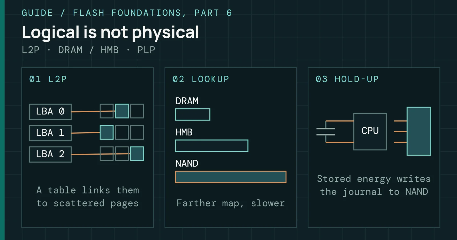
Part 6 built the map, the flash translation layerThe flash translation layer is the firmware that maps host addresses to physical flash locations and hides the rules of erase blocks and wear. (FTL). This part covers GC and wear levelingWear leveling spreads erases evenly over all blocks. Dynamic leveling picks young blocks for new writes, while static leveling also moves cold data off them., which are the two jobs that keep that map usable as the drive ages. These background processes decide whether the drive you validated on day one is still the same drive on day one thousand.
GC and wear leveling work behind the spec sheet. Their extra writes pull down performance and shorten drive life, as Park and colleagues put it for write amplification. That extra work shows up in telemetry as write amplification, spare capacity and latency. How much work does a drive do that the host never asked for, and what does that cost in speed and in life? By the end of this part you can read write amplification, spare capacity and latency to answer that, and spot the pattern early enough to plan the fix instead of fighting fires.
Reclaiming blocks that NAND cannot overwrite
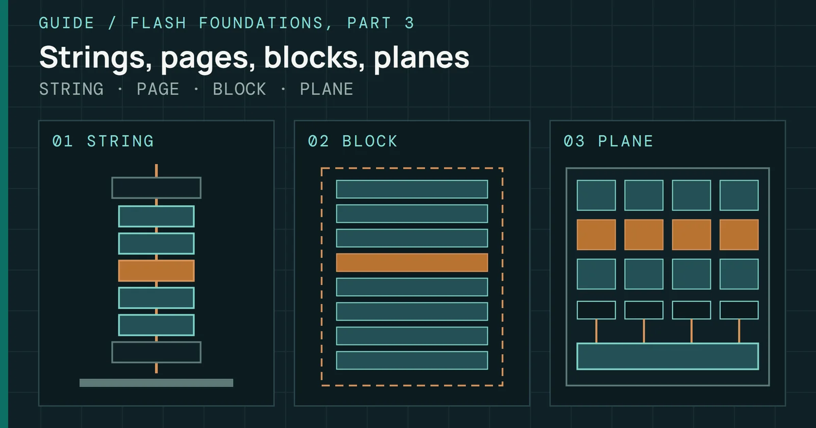
A spinning disk can overwrite a sector, and DRAM can overwrite a cell in place. NAND flash cannot overwrite in place at all. To reuse a page, the firmware must erase the whole block that holds it, because programming only adds charge and removing it takes an erase bias the block shares. Part 3 covers why the erase unit is a block.
This creates an accounting problem. When the host updates a file, the FTL puts the new version in a fresh page and marks the old one invalid. Over time, a drive in active use accumulates blocks holding a mix of valid data and stale copies of data the host has already replaced. Those invalid pages cannot be reclaimed one at a time. They sit, consuming physical space, until the firmware does something about them.
Reclaiming blocks that NAND cannot overwrite
GC copies valid pages out so a whole block can be erased
One victim block through four steps
GC runs four steps on one block (Figure 7.1, victim outlined in copper):
- Selects a victim blockVictim selection picks which block to reclaim. Greedy takes the one with the fewest valid pages, while cost-benefit also weighs how old the data is. (a block with enough invalid pages to be worth reclaiming)
- Copies valid pages out (moves any still-current data to a new location)
- Erases the block (resets all pages to the writable state)
- Returns the block to the free pool (it is now available for new writes)
This runs mostly in the background, triggered by idle time or by free-block headroom running low. Firmware must balance GC work against host I/O so it reclaims space without starving incoming commands.
Write amplification: what every copy costs
GC costs writes, because every valid page copied during a GC cycle is a NAND write the host never requested. Say a 128-page block still holds 100 valid pages. Reclaiming it copies those 100 pages out and frees room for 28 pages of host data. In total the drive makes 128 page programs for 28 host pages, a write amplification factorWrite amplification factor is the data written to NAND divided by the data the host wrote. A value of 1 means no extra internal writes. (WAF) of about 4.6.
WAF measures this cost:
WAF = Total NAND writes / Host writes
Total NAND writes means every byte the drive programs to the media. That covers host data, the SLC staging write and the fold write that follows it (Part 6), GC copies, refresh rewrites and metadata. The OCP Datacenter NVMe SSD specification defines its Physical Media Units Written field this way and requires that it can be used to calculate WAF. This part uses GC-only WAF, which counts relocation alone, when it compares workloads.
Without compression, a WAF of 1.0 is the theoretical floor, because every host write produces exactly one NAND write. Real drives rarely hit it, outside sequential or read-heavy workloads. As a rule of thumb, a GC-only WAF between 1.2 and 1.5 is solid for a well-tuned client drive under mixed workloads. A client drive with an SLC cache can show a total WAF near 2.0 with nothing wrong, because each staged byte is written twice. For a client drive, this page treats a GC-only WAF above 2.0 as a sign of building GC pressure. Enterprise drives run higher by design, and the workload table in In the field shows about 2 to 3 for a 3 drive-writes-per-day (DWPD) class drive and about 5 for a 1 DWPD class drive.
A GC-only WAF of 3.0 means GC and wear leveling alone write three times what the host demands, so two of every three writes are internal housekeeping rather than host data. On a client drive that is a problem. On a 3 DWPD enterprise drive it can be normal. The FTL’s superblock management (how it handles partially filled superblocks under random writes) is a major contributor to WAF, as covered in Part 6.
Spare capacity is the other lever. OP is flash the host cannot address, which GC uses as working space (Part 9 covers it). With less working space, each reclaimed block still holds more valid data, so WAF climbs as OP shrinks.
Write amplification: what every copy costs
WAF falls steeply as overprovisioning grows
Greedy GC, uniform random writes over the full drive, no deletes
Figure 7.2 plots the expected-value model that Park and colleagues published for uniform random writes and greedy GC, with their measured drive marked. WAF falls steeply as OP grows from 5% and flattens above about 35%. The model gives about 7.8 at 7% OP and 2.48 at 28% OP, the two operating points the workload table in In the field uses for heavy random writes. At 28% the same team measured a WAF of 2.466 on a real enterprise SSD, close to the model. That is a single point, but they reached 28% OP by filling part of the drive with cold data that greedy GC does not pick, and the model assumes uniform random writes over the whole drive.
Endurance maps straight to WAF. A terabytes written (TBW)Terabytes written is the total host data a manufacturer rates a drive to absorb over its life under the warranty conditions. rating is based on a specific workload, so it carries a specific total WAF. Workload fit works through what happens when the real workload runs at a different one. Park and colleagues motivate their WAF models by noting that write amplification pulls down performance and reduces the life of the device.
Victim selection: choosing the block that costs least to reclaim
Victim selection decides how efficiently the firmware uses free space and how much valid data it has to move to reclaim it. Four policies cover most designs.
Victim selection: choosing the block that costs least to reclaim
The same four blocks give two different victims
Tags give each block’s invalid share and data age
Two of them are run on the same four blocks in Figure 7.3, using illustrative values. Greedy takes the block with the most invalid pages. Cost-benefit also weighs how old the block’s data is, so it skips a young block that is about to lose more pages anyway and takes an older block with slightly fewer invalid pages.
Greedy selection
Greedy selection chooses the block with the highest proportion of invalid pages. It minimizes the valid data copied per reclamation cycle, and for uniform random writes it is close to optimal. Greedy does worse when some blocks are heavily written and others are rarely touched. Cold blocks with only a few invalid pages rarely get picked, so that stranded space stops acting as OP for hot data. WAF rises unless the firmware separates hot and cold writes.
Cost-benefit selection
Cost-benefit selection weighs the benefit of reclaiming a block against the cost of moving its remaining valid data. A block that is 90% invalid is cheaper to reclaim than one that is 60% invalid. But a block of cold data may be the better target. A block with slightly more invalid pages may hold hot data that will be rewritten soon. Cost-benefit algorithms use block age as a proxy for how soon the remaining data will change. An early flash file system scores a block by multiplying its age (the time since one of its pages was last invalidated) by the free space reclaimed, 1 − u, and dividing by the copy cost, 2u. Here u is the fraction of the block still valid, so copying costs u reads plus u writes.
Age-aware selection
Age-aware selection goes a step further with hot/cold data separationHot data is rewritten often and cold data rarely. Keeping them in separate blocks means blocks empty out together, which reduces garbage collection copying., which controls where data is placed as well as which block gets reclaimed. Cold data that has stayed stable for a long time gets consolidated with other cold data, instead of mixed with hot data that will turn over quickly. When hot and cold data share a block, GC has to copy the cold pages again every time it reclaims that block for hot traffic. Separating the two populations cuts WAF in workloads with strong temporal write locality.
Workload-adaptive selection
Workload-adaptive selection observes access patterns at runtime and adjusts strategy accordingly. A database log workload looks nothing like a video archive, and the optimal GC behavior differs between them. Adaptive algorithms try to match strategy to observed behavior, rather than run a static policy tuned for one workload class and merely adequate for the rest.
This table sets the four policies side by side on selection criterion, workload fit, weakness and WAF tendency.
| Algorithm | Selection criterion | Best workload fit | Weakness | WAF tendency |
|---|---|---|---|---|
| Greedy | Highest proportion of invalid pages | Uniform random writes, or skewed writes once hot and cold data are separated | Strands free space in cold blocks under skew without separation | Near-optimal for uniform writes, rises under skew without separation |
| Cost-benefit | Reclaim benefit versus valid-data copy cost | Mixed workloads with varied write rates | More computationally expensive than greedy | Lower than greedy on mixed traffic |
| Age-aware | Cold block age combined with invalidity | Workloads with strong temporal write locality | Requires tracking data age, overhead in write-heavy scenarios | Significantly lower for cold-data-heavy workloads |
| Workload-adaptive | Runtime-observed access patterns | Diverse or shifting workloads over time | Startup period before model is reliable, risk of misclassification | Variable, depends on how well the model tracks the workload |
Which algorithm runs inside a given drive is invisible to users and rarely disclosed by manufacturers. Its effects show up in sustained write benchmarks. Watch whether the drive degrades gracefully as it nears steady state, or drops off abruptly in a way idle time does not fully reverse.
Every algorithm described above shares one structural limitation. Selection is driven by invalidation, so blocks whose data never changes are rarely picked as victims. Blocks holding cold data sit untouched while write traffic cycles through the rest of the drive. Those two groups end up with very different program/erase (P/E) cycleA program/erase cycle is one write of a block followed by its erase. Each cycle wears the oxide, and the cell type sets how many cycles it tolerates. counts. GC alone cannot fix this asymmetry, which is the job of wear leveling.
Wear leveling: making the whole drive age together
GC reclaims space. Wear leveling distributes write activity across all available blocks so that no subset wears out while others remain nearly fresh.
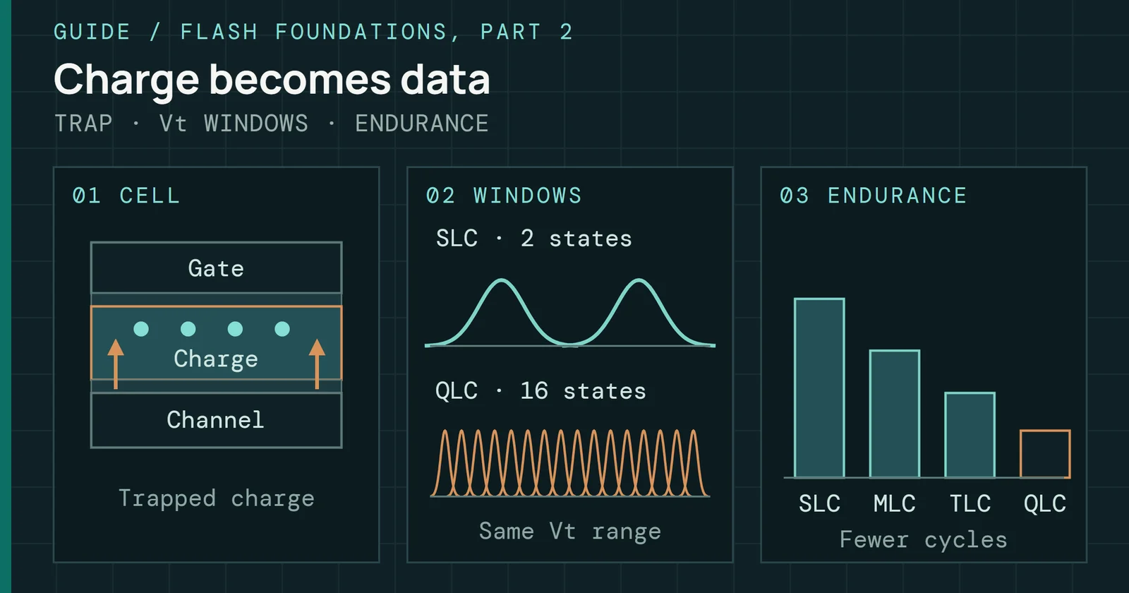
Every NAND block has a finite P/E cycle budget. Part 2 gives illustrative ranges by cell type. Triple-level cell (TLC) in current consumer 3D NAND typically sustains 1,000 to 3,000 cycles and current 3D quad-level cell (QLC) 300 to 1,000, before the raw bit error rate (RBER)Raw bit error rate is the fraction of bits read from the NAND that are wrong before error correction is applied. climbs to the point where error-correcting code (ECC)Error-correcting codes add parity bits to each block of data so the controller can find and fix bit errors on read. cannot reliably correct errors. Part 8 defines RBER. Effective lifespan follows the most-worn blocks instead of the average.
Dynamic wear leveling
Dynamic wear leveling redirects new writes to the least-worn available blocks. The FTL’s logical-to-physical indirection makes this transparent to the host because logical addresses float freely over the physical space, and the controller places data wherever it fits best. Dynamic wear leveling handles hot data well. It leaves cold data anchored in place. Those blocks gain P/E cycles slowly while write traffic moves through the rest of the drive.
Static wear leveling
Static wear leveling addresses cold data directly. Firmware periodically identifies blocks with low erase counts that hold long-unchanged data. It relocates that cold data to higher-wear blocks, freeing the low-wear blocks for active write traffic. This forces the wear distribution to converge across the whole drive instead of only the blocks currently receiving writes. Static wear leveling adds write overhead. Relocating cold data costs write amplification, paid in exchange for more uniform block aging across the full capacity.
The block erasing table is one published design, and it shows how little state this takes. It keeps one bit per set of blocks, set when any block in the set is erased during the current interval. When erases divided by set bits reaches a threshold T, the firmware has GC collect a set whose bit is still zero. None of its blocks was erased this interval, so it likely holds cold data.
Take a worst-case drive with H − 1 hot blocks, C cold blocks and one free block. Each interval then holds T × (H + C) erases, of which C are forced, so static wear leveling adds C / (T × (H + C) − C) extra erases, close to 1/T when cold blocks dominate. For the paper’s 1GB multi-level cell (MLC) example, with H = 256 and C = 3,840, T = 100 adds 0.946% more erases and T = 1,000 adds 0.094%. Each forced erase also copies a cold block’s pages, so the extra page copies run about N/L times the extra erase ratio, where N is pages per block and L is the average number of pages GC copies when it erases a hot block. Choosing T is a trade. In the paper’s simulations a small T gave good gains in time to first block failure, but the authors advise against a very small T, because it triggers static wear leveling often and so adds the most extra erases.
Wear leveling: making the whole drive age together
Static wear leveling pulls every block toward the same wear
Blocks counted by erase count, three drives, same writes
Counting blocks by erase count in three drives (Figure 7.4, illustrative values) shows the effect. With no wear leveling, the blocks that take the writes pile up at the right edge while the cold blocks stay at the left. Dynamic wear leveling evens out the right-hand group only. Static wear leveling pulls the whole population toward the middle, at the cost of the relocation writes described above.
This table compares the two strategies on target, mechanism, P/E distribution and write overhead.
| Strategy | Targets | Mechanism | P/E distribution outcome | Write overhead added |
|---|---|---|---|---|
| Dynamic | Hot data (blocks receiving active writes) | Redirects new writes to least-worn available blocks | Evens wear across actively written blocks, cold data remains in place | Minimal, integrated into normal write placement |
| Static | Cold data (blocks with low erase counts holding stable data) | Periodically relocates cold data to higher-wear blocks, frees low-wear blocks for write traffic | Extends distribution evenness across the full NAND population | Meaningful, forced relocation writes trade endurance headroom for uniformity |
Both strategies operate in concert with GC. When GC selects a victim block and moves its valid pages out, wear leveling influences where those pages land and which free blocks receive incoming host writes. GC and wear leveling are interleaved policies run by the same firmware subsystem.
TRIM: telling the drive which pages are stale
Operating systems delete files. Without additional communication, the SSD does not know this has happened.
A controller treats every written page as valid until the host overwrites that logical address. A file deleted six months ago may still occupy physical NAND pages that GC copies from block to block during reclamation, and all of that copying is wasted work.
TRIM closes this gap. When the host deletes a file, the operating system issues a TRIM command for that logical range, either right away or in a later batch. It marks those physical pages as invalid without waiting for an overwrite. A later GC cycle can reclaim them without paying the copy cost for stale content. TRIM is the AT Attachment (ATA) name for this command. NVMe uses Dataset Management with the Deallocate attribute, and Small Computer System Interface (SCSI), including Serial Attached SCSI (SAS), uses UNMAP.
TRIM is advisory, which means a controller may take no action on the information it receives. The NVMe command set specification asks hosts to send each deallocate range as a multiple of the namespace’s preferred deallocate granularity, starting at its preferred alignment, because that may improve deallocate performance. It does not say what a drive does with a misaligned range. As an inference from mapping granularity (commonly 4KiB), a range that does not cover a whole unit probably cannot unmap it, so a partition misaligned to the drive’s units likely benefits less. TRIM does not free space instantly or erase anything on its own. The controller still decides when to actually erase the blocks that hold those invalidated pages. But it gives GC much better information, and it cuts WAF by skipping work on data that no longer matters.
In enterprise environments with NVMe over Fabrics (NVMe-oF)NVMe over Fabrics carries NVMe commands across a network, such as RDMA, Fibre Channel or TCP, so remote drives look like local ones., hypervisor storage stacks, or storage area network (SAN) arrays between host and drive, TRIM/UNMAP delivery cannot be assumed and needs to be verified end to end.
TRIM: telling the drive which pages are stale
A delete reaches the drive only if every layer passes it on
One delete, five layers, and where each can drop the hint
In Figure 7.5, one delete travels down the stack. Arrays that disable UNMAP pass-through, hypervisors that do not propagate deletion hints, and storage drivers that drop the command all degrade GC efficiency without any visible error. Because the drive never gets a signal that the pages are stale, WAF climbs and performance erodes while the hardware works correctly.
TRIM and UNMAP pass-through support varies widely by environment, as the table shows.
| Environment | TRIM / UNMAP status | Configuration required | Consequence if blocked |
|---|---|---|---|
| Windows 10/11 + NVMe direct-attach, NTFS | Native, automatic | None. Optimize-Volume also retrims a TRIM-capable SSD by default | N/A |
| Linux (ext4, XFS, Btrfs) | Supported, not always default | Mount with discard option or schedule fstrim via cron/systemd | Pages remain marked valid, GC copies stale data, WAF climbs |
| VMware ESXi guest (vSCSI/NVMe) | Automatic on VMFS6 with thin disks | Confirm datastore space reclamation is enabled, unmap must be 1MB or an aligned multiple | Requests under 1MB or misaligned are not processed, so the space is not reclaimed and GC efficiency is degraded |
| Windows Server + Storage Spaces / RAID | Storage Spaces yes, hardware RAID varies by vendor | Storage Spaces typically pass UNMAP through, so check RAID controller TRIM support per level | WAF rise proportional to delete volume, may surface as premature endurance decline |
| NVMe-oF fabric (initiator to target) | Supported, target dependent | Confirm the target advertises Dataset Management (the Optional NVM Command Support (ONCS) bit that carries Deallocate) and its backend passes it to the drive | Target backend absorbs the hint, drive operates without deletion hints |
| SAN array (SCSI UNMAP to backend NVMe) | Vendor and firmware dependent | Must be enabled at array level, confirmed by the logical unit number (LUN) reporting UNMAP support, such as vSphere Storage APIs for Array Integration (VAAI) Delete Status | Backend drives show elevated WAF, array-level thin provisioning reclamation also impaired |
Where TRIM is not enabled at every layer, the drive keeps treating stale pages as valid data, so confirm it at each layer.
Background GC: idle time refills the free pool
A buffer of pre-erased blocks avoids the worst case. That case is a host write that arrives with no free block ready, which forces the firmware to stop and run emergency GC before it can accept the command.
GC scheduling falls into two modes. Idle-time (background) GC runs during windows when no host commands are queued, using NAND bandwidth that would otherwise sit unused. The drive reclaims space proactively and keeps a buffer of pre-erased blocks ready, so the next write burst does not have to wait on the controller to stop and reclaim. Active (foreground) GC runs at the same time as host I/O, competing with host reads and writes for die and channel time. Controllers must arbitrate between GC and host commands. An Intel patent on host-controlled garbage collection states that write bandwidth to the NAND dies is divided between host writes and writes for garbage collection, and that bursty program bandwidth negatively impacts read quality of service.
That patent describes the host triggering controlled GC during IO idle time. A drive under sustained write pressure with little idle time spends more of its GC in the active mode, and the patent ties variable sustained write bandwidth to that split between host writes and GC writes.
Background GC: idle time refills the free pool
Idle time refills the free pool before the next burst
Host activity, GC work and free blocks on one time axis
An SSD idle for several minutes often performs better on the next write burst than one that was writing continuously up to that moment (Figure 7.6). The idle drive ran background GCBackground garbage collection reclaims space during idle time, so that foreground writes do not have to wait for it. and, on a client drive, also folded its single-level cell (SLC) cache (Part 6 covers folding), so it arrived at the burst with free blocks and cache space ready. The continuously written drive may have hit the burst with the free block pool nearly empty.
Background GC rewrites data, which adds wear, especially when it relocates data the host was about to overwrite anyway. How much of it a drive runs is a firmware policy. Users never see that choice, but it shows in how the drive recovers when idle time follows a long write run.
The more consequential scheduling decision is how many dies are programming while the host reads. Per the Intel patent, the chance of a host read colliding with a write depends on the number of NAND dies being programmed at any time. Dies a controller spends on GC programs therefore affect how often reads wait.
Naive firmware relies on the threshold trigger alone, with no idle-time preference. GC then runs while write commands are also arriving, competing directly for die and channel time. The difference between the two approaches does not show up in burst benchmarks. It shows up in the 99.9th percentile latencyA latency percentile gives the time within which that share of commands finished. The 99th percentile is the time that 99% of commands beat. (p99.9, the time within which 99.9% of commands finish) under mixed read/write workloads over hours of sustained load, which is the condition that matters in production. Part 9 covers percentiles, and In the field shows what the pattern looks like in telemetry.
Read disturb and refresh: background writes the host never asked for
GC and wear leveling are the obvious sources of background write activity. Read disturb managementThe controller counts reads per block and rewrites a block into fresh flash before read disturb errors grow beyond what error correction can handle. is the one that surprises engineers who assume a read-dominant workload is easy on a drive.
As Part 3 established, reading a NAND cell biases every unselected wordline in the block to a pass voltage, so the other cells in the string conduct. Applied across tens of thousands of reads to the same block, that stress shifts threshold voltages in unread cells without any intentional write ever occurring. Given enough read cycles against the same physical block, bit errors emerge from pure read traffic.
Blocks that are only partly programmed are more exposed. At the 2015 Flash Memory Summit, an IBM characterization of NAND flash reported read disturb much worse on partially programmed blocks than on fully programmed ones. Pages programmed after the reads came out degraded, and the erased state was affected dramatically, and an erase resets the effect.
Firmware keeps a read counter for each block. When that count crosses a threshold, which a read-reclaim study modeled at 40,000 to 200,000 reads and which varies with NAND generation and cell type, the firmware schedules a refresh for the block. Refresh means reading every page, writing the data to a new physical location, and erasing the original block. The data is valid and unchanged, yet the drive writes it again because data left on stressed cells will eventually pick up errors. Firmware literature calls this read reclaim. That study also proposed a design called redFTL, which moves read-hot data to blocks read at a lower voltage, which resist disturb better. It depends on NAND modified to support more than one read mode, and it trades write speed for that resistance. The authors’ evaluation found it cut the execution time overhead of read-disturb management by 73% compared with conventional read reclaim.
Read disturb and refresh: background writes the host never asked for
A read counter turns pure reads into background writes
One block from its first reads to its erase
This refresh work competes with GC for NAND channel time, as Figure 7.7 shows for one block from its first reads to its erase. Both processes read pages, write data to new locations, and erase blocks. Both run in the background, and both usually yield to host commands. Sustained reads against a narrow address range trigger extra refresh work. Examples include hot data that misses host-side cache, cold storage under audit, or a drive serving as a read-optimized tier. Refresh scheduling then generates write activity the host never sees, in a workload that looks write-idle from the outside.
RefreshRefresh and scrubbing read old data in the background, correct errors and rewrite it, so charge loss does not accumulate unseen. also exists for retention as well as read disturb, and there it can cost a lot of the P/E budget. Early work on planar flash showed two ways to do it. Remapping refresh rewrites the data to a new block, which spends a full program/erase cycle each time. In-place refresh tops up the charge on the same cells without erasing and so spends far less, but it only works on cells that lost a little. The same work found that the shorter the retention promise, the more cycles a cell can take: a drive that refreshes data every few days can be rated for many times the cycles of one that must hold data for years. On 3D charge-trap NAND, charge can also leak out of the trap in three dimensions. Luo’s 2018 Carnegie Mellon thesis states that this extra leakage lasts only a few seconds after programming, after which long-term retention resembles planar NAND. Measurements on 3D chips show the loss unfolding over a longer span: Part 8 covers retention errors that rose tenfold within about 3 hours and tenfold again by about 11 days.
Keeping write-hot data apart from cold data helps here too, because data that is rewritten constantly never needs refreshing. In the write-hotness-aware retention management (WARM) study, under 1% of pages took most of the writes in all but one of the workloads, and pairing WARM with adaptive refresh gave 1.21 times the average lifetime of adaptive refresh alone, in tests on planar parts.
A drive showing background wear in a read-dominant deployment is not necessarily misconfigured or failing. It may be doing exactly what its firmware is designed to do. It may be refreshing stressed blocks before read disturb pushes errors past what ECC can correct. The Media and Data Integrity Errors count in the NVMe Self-Monitoring, Analysis and Reporting Technology (SMART)The SMART and NVMe health log reports counters such as temperature, percentage used, available spare, media errors and data units written. / Health Information log should stay at zero. The NAND write count (the Open Compute Project (OCP) Physical Media Units Written field; the standard NVMe log reports only host writes as Data Units Written) will not. Track media writes per day alongside host writes. Media writes that continue for days with near-zero host writes point to refresh or other background relocation rather than SLC folding. Folding only moves data the host already wrote and stops when the SLC cache is empty, as Part 6 describes. Refresh follows reads and time, so it keeps going. The OCP SMART Cloud Attributes log page (0xC0) reports Refresh Counts, the blocks reallocated to maintain data integrity, and its definition excludes space created by garbage collection, which tells the two apart.
Block retirement: the other wear curve
WAF measures how hard the firmware is working to manage available space. Block retirement rateThe block retirement rate is how quickly blocks are removed from service. A rise signals that the flash is wearing out faster than expected. measures how fast the usable block pool is shrinking.
Most NAND dies ship with some blocks that failed factory testing. These are factory bad blocks, which the firmware finds and skips and never presents to the host as usable capacity. They are a normal product of the yield distribution and do not indicate a defective drive. Part 6 covers how bad blocks are tracked.
Grown bad blocks appear during service life. As cells build up P/E cycles and oxide degrades, individual blocks eventually fail a program or erase operation, or exhibit error rates that exceed what ECC and read retry can reliably address. The firmware retires them. It removes them from the active write pool, logs the retirement event and substitutes a block from the overprovisioned reserve. The Available SpareAvailable Spare is a health value showing the percentage of spare blocks remaining. The drive warns when it falls below a set threshold. field in the NVMe SMART / Health Information log tracks this reserve. It starts at 100% on a new drive and declines as reserve blocks are consumed to replace retired ones.
A healthy drive’s block retirement curve is slow and predictable. Retirements track write volume. Available Spare declining at a rate consistent with the drive’s write history and cell type is normal.
Block retirement: the other wear curve
Accelerated retirement reaches the threshold much sooner
Healthy and accelerated drives against one warning threshold
Two drives run against the same warning threshold in Figure 7.8, drawn as illustrative curves. The accelerated drive reaches it with far fewer terabytes written, because Available Spare is falling faster than write volume predicts, and that means blocks are retiring early.
Possible causes:
- Workload mismatch, with WAF above what the endurance rating assumed
- Sustained heat, which speeds retention loss and raw bit error growth
- A cluster of failures from a yield-marginal die region
Divide spare consumed by Data Units Written to get a retirement rate. Each unit is 512,000 bytes (512 bytes times 1,000), so convert to terabytes first. Power-on hours give the rate per month. In a fleet, flag any drive using spare much faster than its cohort at the same write volume. Investigate before it reaches the Available Spare Threshold.
When Available Spare falls below the Available Spare Threshold, the drive sets the spare bit in the Critical Warning field. The bit marks a warning rather than a failure, and it tells the host the reserve block pool has dropped below the warning level, so the drive has less room to retire failing blocks. Start migrating data and schedule replacement here. A drive that hits the threshold early because of accelerated retirement rather than normal aging may keep losing blocks at that pace, so its remaining life is uncertain.
Workload fit: matching the rating to the deployment
Understanding GC behavior changes how drive selection should work. The question shifts from comparing spec sheets to checking workload fit.
A database transaction log writes small sequential records at a high, steady rate, and recycles its segments as they fill. It is hard on endurance because of sheer write volume, even though its WAF stays moderate. New data drains the free block pool fast. The hot region is narrow, so most of the drive holds cold data, and wear leveling has to keep moving that cold data to spread wear. The firmware spends heavy bandwidth on reclamation to keep headroom. Seagate’s over-provisioning guide suggests raising OP to 20-28% on enterprise SSDs used in high-write environments. A transaction log is such a high-write use, and the extra spare area gives GC free blocks to work with ahead of the host writes.
A read-dominant analytics archive writes large sequential blocks infrequently and spends most of its time reading. GC pressure is low, and the SNIA endurance white paper puts WAF close to 1 for sequential workloads. In my judgment, extra OP adds cost here without much benefit, so a QLC drive with minimal OP fits.
A mixed enterprise workload is the hardest case to predict. It might mean virtualized storage with diverse tenants, databases with balanced read/write ratios, or application servers with irregular I/O. GC behavior under mixed load depends on write locality, delete frequency, queue depth, and how read and write commands interleave. Drives that perform alike in single-workload benchmarks can diverge widely under mixed load, because GC scheduling interacts differently with varied write traffic patterns.
A common field mistake is sizing drives on capacity and rated throughput without considering workload-specific WAF and its effect on TBW consumption. A drive rated for 1,200TBW at an assumed total WAF of 1.5 will wear out long before the host writes 1,200TB, if it actually runs at a total WAF of 3.0.
Workload fit: matching the rating to the deployment
Doubling the real total WAF halves the host writes a rating allows
Host writes before wear-out for a drive rated at total WAF 1.5
As a share of the rating, that example looks like Figure 7.9. The rating fixes a budget of media writes at the assumed total WAF, so the host writes the drive can absorb fall in inverse proportion to the total WAF it actually runs at. At a total WAF of 3.0 the drive reaches wear-out at half the rated host writes. The rating itself was honest, but the workload assumption did not match the deployment. Part 9 covers what endurance ratings assume. Checking WAF and GC behavior before procurement prevents this class of problem.
In the field: reading WAF, latency and spare
For engineers tracking fleet health, WAF is a diagnostic signal as much as an efficiency metric. Under a stable workload, WAF should converge to a predictable steady-stateSteady state is the condition where performance has stopped changing because the drive is full of data and garbage collection runs continuously. value, the condition where performance has stopped changing because the drive is full of data and GC runs continuously (Part 9 defines it).
That value depends heavily on workload type. Where a source states a value the row cites it. The database log row is a rule of thumb:
| Workload | Typical steady-state GC-only WAF | Notes |
|---|---|---|
| Read-dominant (analytics archive, cold storage) | About 1 | Little valid data to move during reclamation. The SNIA endurance white paper puts WAF close to 1 for a drive under about 60% full with TRIM |
| Sequential write (video ingest, backup streams) | About 1 | Near-ideal GC conditions, blocks fill completely before reclamation is needed |
| Database transaction log | 1.3–2.0 | Sequential bursts at sustained rates, segment recycling keeps WAF moderate |
| Mixed enterprise (virtualized, application servers) | 2–3 for a 3 DWPD class drive; about 5 for a 1 DWPD class drive | Both SNIA figures. Varied write traffic increases GC scheduling complexity, and the 1 DWPD drive has less spare area |
| Heavy random small-block write (online transaction processing (OLTP), small random updates) | 2.466 measured at 28% OP, reached by filling the drive with cold data; about 7.8 at 7% OP from the same paper’s model (uniform random writes over the whole drive) | Blocks fill with scattered valid data, page migration cost rises sharply as overprovisioning shrinks |
Once a system settles into its workload’s expected range, WAF should stay fairly consistent from week to week. These ranges assume adequate overprovisioning and functioning TRIM. They are GC-only WAF. They leave out the SLC staging and fold writes covered in Part 6, which add up to 1.0 at most on a drive with an SLC cache, and any refresh rewrites. Add them when you compare against a total measured from the OCP log. A drive running well above its workload’s expected range needs a closer look.
When WAF drifts upward from an established baseline without a workload change, first confirm that TRIM still reaches the drive. If it does, the drive’s internal state is changing, for one of these reasons:
- The free block pool shrinking faster than GC can replenish it
- Cold data thrash from excessive static wear leveling relocations
- Block retirement speeding up as marginal blocks fall below quality thresholds
End-of-life behavior maps directly to GC state. Drives that age gracefully show a gradual WAF increase as the free block pool tightens and GC works progressively harder to maintain headroom. Drives that fall off a performance cliff show WAF spiking sharply as block retirement accelerates and the firmware begins emergency reclamation to avoid running out of writable space. The firmware shifts from routine housekeeping to crisis response, and tail latency climbs with it.
In the field: reading WAF, latency and spare
A graceful drive drifts up; a cliff drive stays low, then spikes
Two end-of-life paths on the same axes
Two end-of-life paths share the axes in Figure 7.10 (illustrative values). The teal curve rises gradually. The copper curve stays low until the free block pool runs out, then climbs sharply.
GC-induced performance effects appear in latency percentile data before they are visible in throughput numbers. A drive handling GC pressure well shows occasional p99.9 latency spikes while p50 latency (the median) stays low. These spikes are expected because a command occasionally lands on a die that is busy with a program or erase that reclamation already started, and it waits for that operation to finish. Brief spikes are normal, but sustained elevation is a problem.
A problem shows as p99.9 latency staying elevated across the entire observation window, or p50 latency drifting upward over weeks without a workload change. When either pattern appears in production telemetry, and thermal throttling, read-retry growth, and host-side causes are ruled out, the drive has likely entered a state where GC overhead is no longer confined to occasional interruptions. The firmware is trading latency for reclamation work because the free block pool cannot absorb the write rate without continuous intervention.
Broken TRIM is the preventable version of this problem. When a hypervisor setting, driver quirk, or array config silently drops TRIM, the controller works from stale information, WAF rises, and sustained performance falls well below what the same hardware delivers with TRIM intact. Spare consumption is the second signal to trend alongside WAF, and block retirement shows how to turn it into a rate.
Fleet telemetry makes this visible at scale. A WAF proxy boxplot by drive class makes outliers easy to spot. The outliers are drives running much higher WAF than their cohort in the same deployment. A drive well above its cohort’s upper whisker in a stable fleet is worth pulling for analysis before the host sees an error. The pattern can appear well before the drive reports an uncorrectable error.
What GC and wear hand to error correction
The internal writes from GC, wear leveling and refresh wear the cells exactly as host writes do, and WAF is the number that counts them. Host-managed designs such as Zoned Namespaces and Flexible Data Placement move part of that work to the host, and Part 10 covers them.
What GC and wear hand to error correction
Garbage Collection & Wear feeds 2 later parts.
Arrows run to the parts that build on this one.
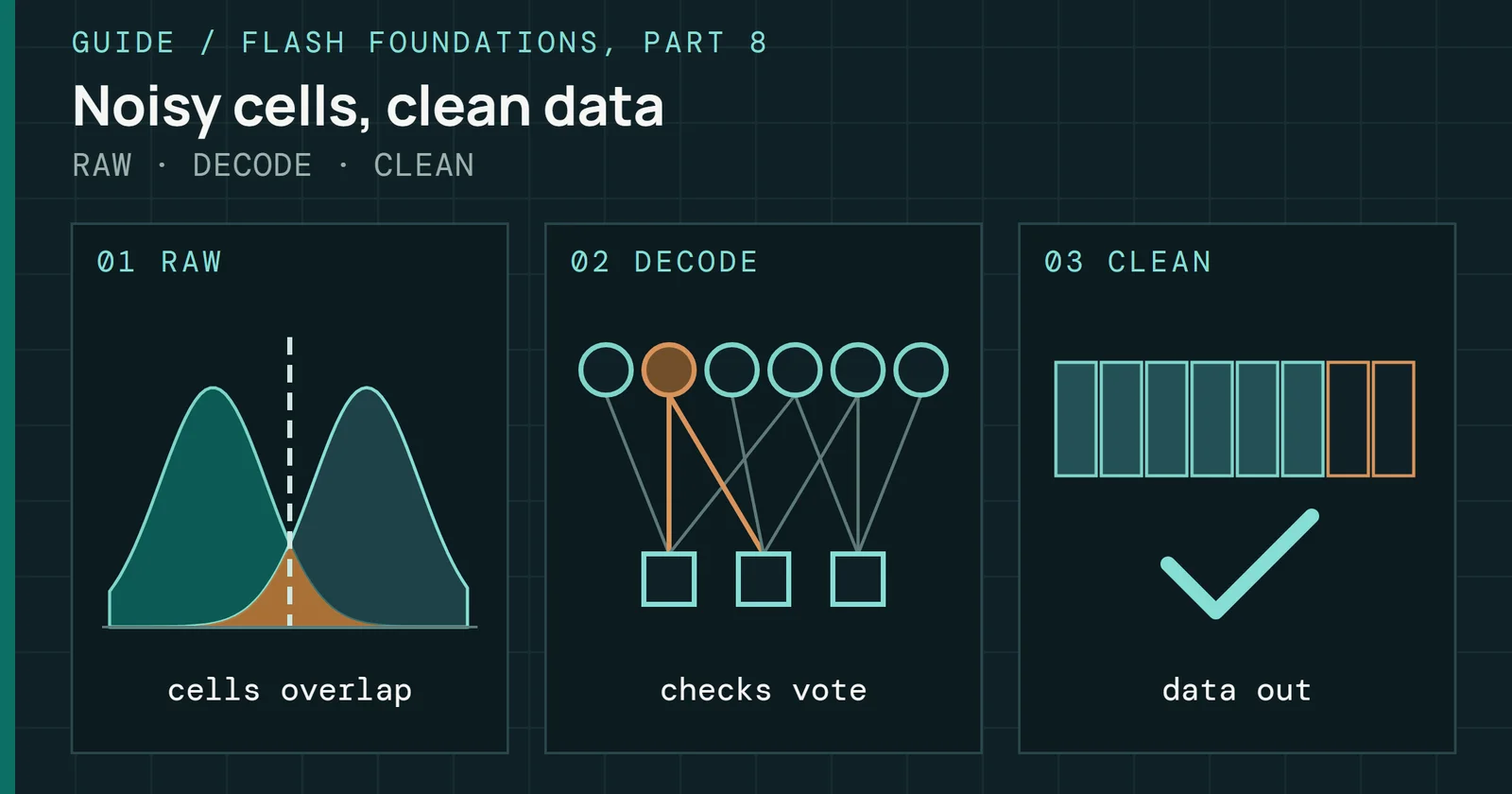
Part 8 covers what happens when that wear starts flipping bits. It traces how error correction grew from Hamming codes to soft-decision low-density parity-check (LDPC)LDPC is a code whose decoder passes confidence messages back and forth until the errors resolve. It corrects more errors than BCH, especially with soft input. decoders that make dense modern NAND viable.
Sources
Primary is the original paper, standard or datasheet. Secondary is a review, a vendor summary or a news report. Measured is my own test data.
Show all 30 sources, 26 primary
- PrimaryA Flash-Memory Based File SystemUSENIX Winter 1995 Technical Conference, 1995
- PrimaryEndurance Enhancement of Flash-Memory Storage Systems: An Efficient Static Wear Leveling DesignACM/IEEE Design Automation Conference (DAC), 2007
- PrimaryAnalytic Modeling of SSD Write PerformanceACM SYSTOR 2012
- PrimaryFlash Correct-and-Refresh: Retention-Aware Error Management for Increased Flash Memory LifetimeIEEE ICCD 2012 (author copy on figshare, Carnegie Mellon University), 2012
- PrimaryRead Disturb Errors in MLC NAND Flash Memory: Characterization, Mitigation, and RecoveryIEEE/IFIP DSN, 2015open copy
- PrimaryWARM: Improving NAND Flash Memory Lifetime with Write-hotness Aware Retention ManagementIEEE Symposium on Mass Storage Systems and Technologies (MSST), 2015
- PrimaryAn Integrated Approach for Managing Read Disturbs in High-Density NAND Flash MemoryIEEE Transactions on Computer-Aided Design of Integrated Circuits and Systems, 2016
- PrimaryFlash Reliability in Production: The Expected and the UnexpectedUSENIX FAST ’16, 2016
- PrimaryPractical Implication of Analytical Models for SSD Write AmplificationACM/SPEC ICPE 2017, 2017
- PrimaryArchitectural Techniques for Improving NAND Flash Memory ReliabilityCarnegie Mellon University (PhD thesis), 2018
- PrimaryUS12340113B2 - Host controlled garbage collection in a solid state driveGoogle Patents, 2021
- PrimaryNVM Express NVM Command Set Specification, Revision 1.0dNVM Express, Inc., 2023
- Primary28.5. WAL ConfigurationPostgreSQL Documentation, 2026
- PrimaryEndurance of NVMe, SAS, and SATA SSDsSNIA
- Primaryfsutil behaviorlearn.microsoft.com
- PrimaryHeatWatch: Improving 3D NAND Flash Memory Device Reliability by Exploiting Self-Recovery and Temperature Awareness
- PrimaryImproving 3D NAND Flash Memory Lifetime by Tolerating Early Retention Loss and Process Variation (Luo et al., SIGMETRICS 2018; arXiv:1807.05140)arXivopen copy
- PrimaryNew API allows apps to send TRIM and Unmap hints to storage mediaMicrosoft Learn
- PrimaryNVM Express Base Specification, Revision 1.4cNVM Express
- PrimaryNVMe Cloud SSD SpecificationOpen Compute Project
- PrimaryOptimize-Volume (Storage)learn.microsoft.com
- PrimarySpace Reclamation Requests from Guest Operating Systems (VMware vSphere 8.0)Broadcom TechDocs
- PrimaryStorage array space not reclaimed after Guest OS cleanup on VMFSknowledge.broadcom.com
- PrimaryThe Design and Implementation of a Log-Structured File Systempeople.eecs.berkeley.edu
- PrimaryTiny-Tail Flash: Near-Perfect Elimination of Garbage Collection Tail Latencies in NAND SSDsusenix.org
- PrimaryTrim/discard — BTRFS documentationbtrfs.readthedocs.io
- SecondaryRead Disturb Characterization for Next-Generation Flash SystemsFlash Memory Summit, 2015
- SecondarySSD Endurance and HDD WorkloadsWestern Digital, 2023
- SecondaryIn-place Switch: Reprogramming based SLC Cache Design for Hybrid 3D SSDsarXiv, 2024open copy
- SecondaryComparing NAND Flash Technology: SLC, MLC, TLC, and QLC for Industrial ApplicationsLexar Enterprise, 2026