A roadmap slide is not a product, and neither is a sample or a demonstration. Part 9 showed what the whole stack delivers against its spec sheet. This part looks forward from that stack and asks which directions you can buy.
Flash Foundations
Flash Foundations, Part 10: The Future of Flash
Sort each direction in flash as on sale, in qualification or in research, and learn what to specify today.
On this page 25 sections
For most of flash history the firmware layer was static. Engineers tuned garbage collection and read retry for the median drive, validated the result against representative benchmarks, and released logic that ran the same on day one and day one thousand. No single setting fits every drive, because dies, workloads and wear states differ. Vendors are moving to adaptive firmwareAdaptive firmware changes its behavior as the drive ages, for example by adjusting read voltages and refresh rates from measured conditions. that observes each drive and tunes itself, while other work shifts data placement to the host, attaches memory over Compute Express Link (CXL)CXL runs over the same physical layer as PCIe but adds cache-coherent memory access, so it moves cache lines rather than blocks of storage., raises link speeds, and packs more bits into each cell. Every one of those directions changes who manages the data or where it sits. None of them changes the NAND underneath.
Which directions can you buy today, which are still being qualified, and which are research? By the end you can sort a roadmap claim into one of those groups and say what it depends on. Dated claims are fenced “As of October 2026”. Memories built to sit beside NAND, including Optane, which went on sale and ended, belong to Beyond NAND.
Machine learning in SSD firmware
Machine learning (ML)Machine learning in firmware uses small trained models to predict things such as the best read voltage or the next access, in place of fixed tables. in SSD firmware is narrower in drives on sale than the research literature suggests. As of October 2026, four techniques run from production to research, and they share one loop. Figure 10.1 shows the loop. The drive observes itself, then a table, a heuristic or a model decides what to do, the firmware acts on a threshold or a garbage collectionGarbage collection copies the valid pages out of mostly stale blocks and erases those blocks, so there is always free space for new writes. (GC) choice, and the result feeds the next observation.
Machine learning in SSD firmware
Adaptive firmware closes a loop that static firmware leaves open
Telemetry, a decision, an action, and a check on the result
Static firmware stops after the third step and repeats the same decision. Adaptive firmware keeps the fourth step, so the decision can move with the NAND, the workload and the wear state. A trained model changes only how the second step decides. It extends the heuristics of victim selection in Part 7 and the read retry in Part 8, and it leaves the domain knowledge behind them in place.
Workload classification
Vendors describe workload-adaptive behavior in current consumer and enterprise controllers. Firmware watches access patterns (sequential or random, read-heavy or write-heavy, bursty or sustained) and adjusts GC aggressiveness and read-ahead depth, and on client drives it also adjusts the single-level cell (SLC) cache allocation. Vendors don’t document how much of this is trained inference and how much is simple pattern detection, so the depth of the production behavior is unknown. One controller vendor is specific about the goal. Microchip’s Haija said in a 2022 EE Asia article about the Flashtec NVMe 4016 that an SI engine in the controller lets NAND management algorithms adapt in real time to the workload the SSD sees.
Adaptive read thresholds
Part 8 explains read retry, which tries alternate read reference voltages when the first read has more bit errors than the error-correcting code (ECC) can fix. Some controllers learn good positions for specific blocks over time, which is learning at block granularity. Vendors publish neither the retry tables nor how they update them, so which drives do this, and how much, is unknown.
Predictive GC
Research has studied the idea at length (a 2019 HotStorage paper is one example), yet no vendor publicly documents it in firmware on sale. One Samsung research paper cut write amplification (the write amplification factor, WAF) by up to 43.5% in its best case, where a neural network predicted each write’s future data temperature and a clustering step sent data of similar predicted temperature to the same NAND blocks.
On-device training
Here the model updates itself from runtime data instead of arriving pre-trained from the factory. Training hardware costs controller die area, and a model that changes itself in the field is hard to validate. This form shows up in research papers and conference talks, and it is the least likely to be in a drive a customer can buy. The table sets the four side by side for a buyer.
| Technique | Status, as of October 2026 | What it needs from the controller (editorial reading) | Observable benefit |
|---|---|---|---|
| Workload classification | Vendors say production, depth not public | Standard controller CPU cores with monitoring logic | Better sustained performance on variable workloads, less unnecessary GC |
| Adaptive read thresholds | Vendors say production in some drives, tables not published | Standard ECC engine with per-block calibration memory | Fewer internal read retries and lower tail read latency |
| Predictive GC | Research, no public production use | Higher CPU capability, more memory for model state and write history | Up to 43.5% lower WAF in the best published case |
| On-device training | Research or early qualification | Dedicated ML training and inference silicon, substantial on-chip static RAM (SRAM) | Continuous per-drive adaptation, not available in purchasable products |
For a buyer the consequence is narrow. The first two techniques are behavior to expect and measure. The last two are not yet a reason to choose a drive.
Zones, placement hints and keys decide who owns the map
Three NVMe extensions move mapping work between the drive and the host. A conventional SSD’s flash translation layer (FTL)The flash translation layer is the firmware that maps host addresses to physical flash locations and hides the rules of erase blocks and wear. owns the map from host addresses to physical NAND (Part 6 covers why), the placement of writes, and GC.
Zoned namespaces and flexible data placement
Zoned Namespaces (ZNS)Zoned Namespaces split the drive into zones that must be written in order, which moves data placement to the host and removes most garbage collection. split a namespace into zones that the host must write in order and reset as a unit, and Part 1 lists the command set. Flexible Data Placement (FDP)Flexible Data Placement lets the host direct writes into separate groups of blocks by lifetime, which lowers garbage collection work without changing the block interface. keeps the ordinary block interface and lets the host tag writes with a placement handle, and Part 6 covers how lifetime hints cut write amplification. Figure 10.2 compares who does the work under each design.
Zones, placement hints and keys decide who owns the map
ZNS moves the most work to the host, and FDP moves less than ZNS
Mapping, placement and garbage collection under three designs
A conventional drive guesses lifetimes and runs GC itself. FDP leaves the map and GC with the drive and supplies the lifetime information the FTL lacked. ZNS goes further. Because the host guarantees sequential writes inside each zone, the drive can use a much simpler map, and GC moves to the host, which copies live data out and resets whole zones. The drive no longer relocates user data to reclaim space. It still runs background media management, including refresh, so it is never idle. Lower write amplification under ZNS follows from this shift in ownership.
Western Digital’s Ultrastar DC ZN540 data sheet describes a 2.5-inch U.2 ZNS SSD aimed at cloud and storage-system builders that can modify their host software, and as of October 21, 2026 the reseller Advanced HPC lists it, in capacities up to 8TB, on a request-a-quote page that shows no price or stock. Meta, Google and Samsung took a related path with FDP, ratified as Technical Proposal 4146 in late 2022. They wanted much of the locality benefit of ZNS with far less host software change. In a kernel storage discussion an engineer from Meta reported that every SSD the company buys has FDP, though it isn’t enabled by default, and hyperscale data placement work has leaned toward FDP.
ZNS needs a zone-aware host, because the file system, database or application has to generate the sequential writes it expects. Linux’s XFS, btrfs and f2fs handle zoned devices natively, and the ZNS authors built a zone-aware backend called ZenFS and ran RocksDB directly on a ZNS SSD through it. Any stack without that support gets no benefit. A reseller lists the drive, but availability is unconfirmed. Microchip’s Haija said in a 2022 EE Asia article that ZNS has had limited traction mainly because of the higher-level pieces needed to make it work at scale, and that SSD and application providers need standards, tools and drivers for more data centers to adopt it. For an enterprise team choosing a platform today, ZNS is worth tracking but not yet worth writing into a specification.
Key value: moving the key index to the drive
NVMe’s Key Value (KV) command set, introduced with NVMe 2.0, exposes store, retrieve, list, delete and exist operations by key. Normally the host writes key-value data to a block device and keeps its own map of keys to block addresses. In a log-structured merge (LSM) tree store such as RocksDB, memtables, Bloom filters and block indexes locate keys in sorted string table (SSTable) files, the file system maps those files to block addresses, and the FTL maps blocks to NAND. Three mapping layers sit between the key and the NAND, and Figure 10.3 shows what a KV drive does to them.
Zones, placement hints and keys decide who owns the map
A KV drive takes the key map off the host
The mapping layers in a key-value store, with and without KV
A KV drive keeps the key index itself, so the host no longer maintains or consults a key-to-block map. Physical placement inside the drive stays with the FTL.
Don’t confuse this command set with the large language model (LLM) “KV cache” that some vendors market SSDs for. They share only an acronym. A prototype Samsung described in 2019 is the KV SSD hardware this page can source. Adoption also needs applications written or ported to issue KV operations instead of block I/O, as with ZNS.
Specification changes
As of October 2026, NVM Express published its 2.4 set of specifications on August 4, 2026, updating all eleven documents (Part 1 lists the set). Three command sets were ratified on July 31: ZNS at revision 1.5, KV at revision 1.4, and Computational Programs at revision 1.3. No new technical proposal for any of the three appears in the revision changes document, and they moved only through engineering change notices shared across the whole set. New proposals went into the Base specification and other documents instead, including PCIe bandwidth and IOPS quality of service, subsystem migration, post-quantum cryptography enhancements and a device voltage monitor. That document also gives notice that the August 2027 release plans to obsolete Predictable Latency Mode and NVM Sets. Standards upkeep continues, and the gap remains host software.
CXL after several revisions, with the ecosystem still maturing
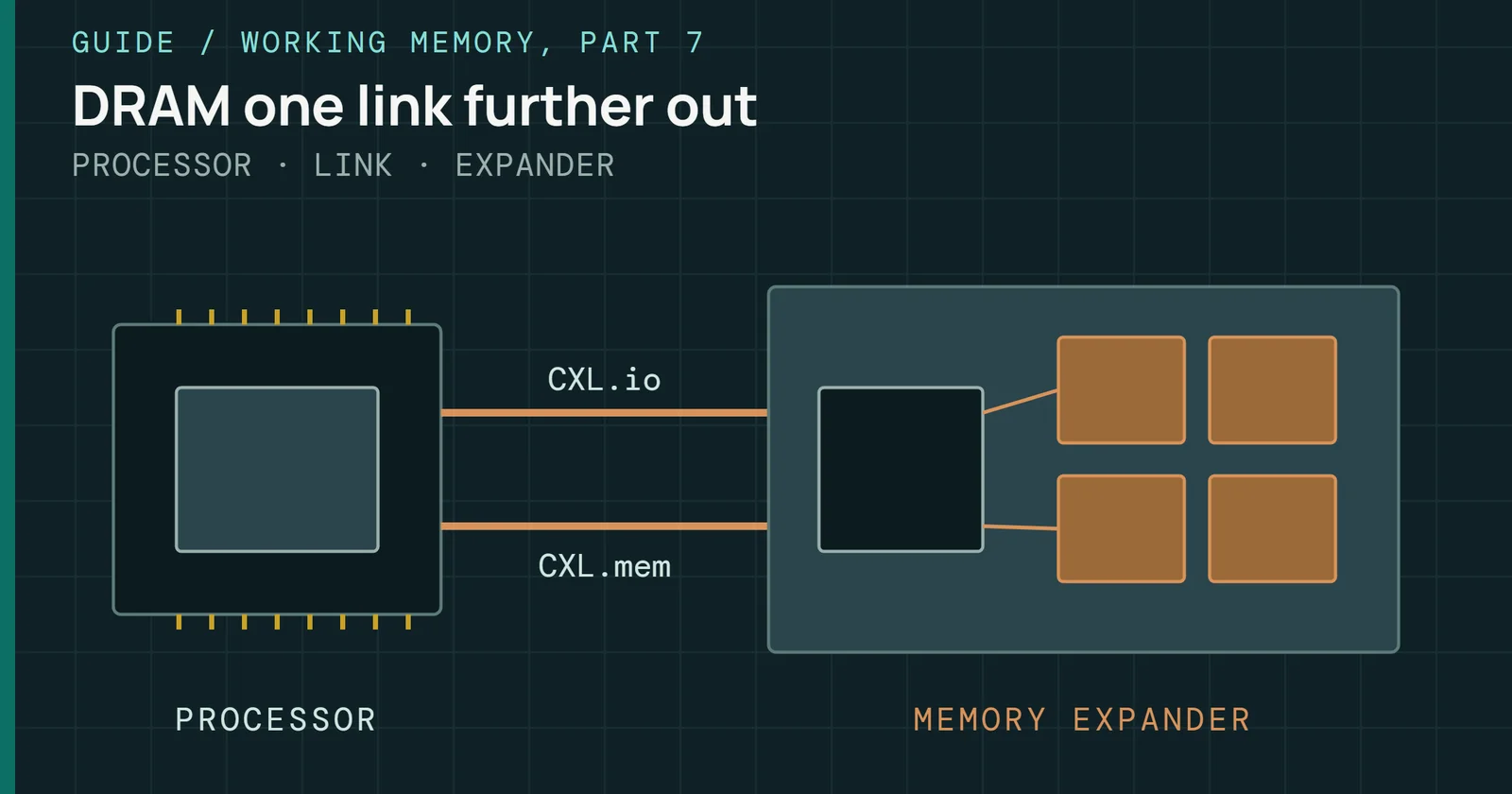
Part 1 covers what CXL is. CXL runs over the same PCIe wires NVMe uses, carrying cache-coherent load and store access to memory instead of block commands. It also covers the trap in the drive bay, where a CXL memory module can sit in an NVMe slot. Figure 10.4 repeats the one difference that matters for this part.
CXL after several revisions, with the ecosystem still maturing
The same bay can hold block storage or load/store memory
An NVMe SSD and a Type 3 CXL memory module on one PCIe link
Panel two’s module has no FTL and never appears as an NVMe namespace. For latency-sensitive access patterns it takes data off the block I/O path, and today that data is mostly DRAM expansion. So the question for storage planning is whether a given deployment is short of memory capacity or short of storage.
As of October 2026, CXL has reached revision 4.0 (November 2025), and what matters is where in the stack adoption has happened. Memory expansion devices (Type 3) are in production servers. AMD’s EPYC 4th Gen (Genoa) supported Type 3 expansion at launch, and Intel’s official Type 3 support arrived later, with 5th Gen Xeon (Emerald Rapids). Lenovo’s CXL 2.0 memory primer puts CXL 2.0 memory support on its ThinkSystem V4 servers with Intel Xeon 6 and expects future AMD EPYC processors to support CXL memory. AMD’s own EPYC 9005 (Turin) data sheet cites CXL 2.0 capabilities for memory-intensive tasks without spelling out Type 3 expansion.
Pooling is earlier. XConn announced early production samples of its Apollo CXL 2.0 switch in March 2024, and the CXL Consortium’s FMS 2025 demo list shows an XConn CXL 2.0 switch sharing a memory pool across hosts. In September 2026 Astera Labs said its Leo 2 P-Series for pooling and sharing, with the rest of the Leo family, is sampling with hyperscaler customers, and in November 2025 it described Leo-based CXL memory expansion in a Microsoft Azure M-series preview.
CXL 3.x is further back. The same demo list shows a Panmnesia cluster with CXL 3.x switches as a demonstration. AMD has announced a 6th Gen EPYC (Venice) as its first PCIe 6.0 server CPU. StorageReview reports that Venice supports CXL 3.1 and that its SP7 platforms are due in Q4 2026, and no CXL 3.x platform is confirmed on sale. The table below pairs each version with the platform it needs. The platform and implication columns are an editorial reading, and the deployment column follows the sources above.
| CXL version | Memory semantics | Deployment, as of October 2026 | Platform needed | Storage implication |
|---|---|---|---|---|
| 1.1 | Type 3 memory expansion | Production | Intel 5th Gen Xeon (Emerald Rapids) or later, AMD EPYC 4th Gen (Genoa) or later | Byte-addressable memory expansion |
| 2.0 | Type 3 expansion, pooling through a CXL switch (tree topology) | Expansion supported on Xeon 6 servers; pooling silicon sampling with hyperscalers (Astera Labs, September 2026) | Xeon 6 or later, plus a CXL switch for pooling | Memory pools allocated to several compute nodes |
| 3.x | Multi-level fabric topology | No CXL 3.x platform confirmed on sale; switches shown in demonstrations; Venice SP7 platforms due Q4 2026 (StorageReview) | Full ecosystem alignment | Fabric-attached memory pooling, not yet deployed |
For most enterprise environments, CXL isn’t yet a storage architecture decision. Fully exploiting CXL 2.0 pooling needs specific processor and platform support, and most enterprise fleets still run on older platforms. If a customer asks whether to build storage architecture around CXL, the field engineer’s answer is not yet for storage and yes for memory capacity. Qualify CXL-capable platforms where a workload needs more memory than the dual in-line memory module (DIMM) slots give. Don’t make a deployment depend on CXL if it must also run on older servers without native CXL support.
PCIe 6.0 and 7.0 signal at the edge of the channel
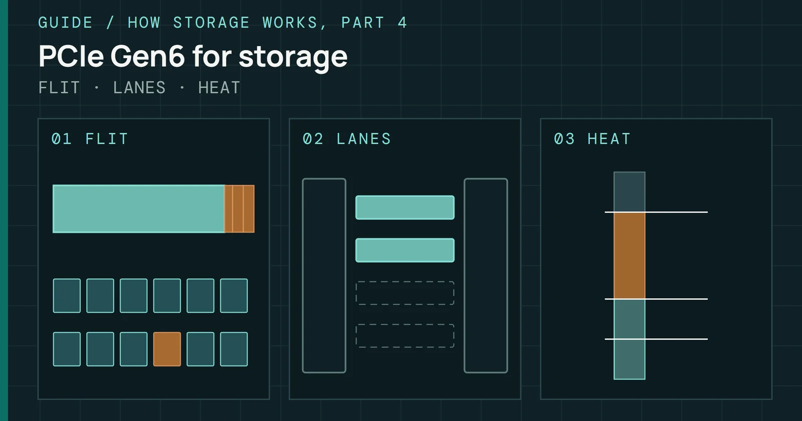
Part 1 gives the generation ladder. PCIe 6.0PCIe 6.0 uses PAM4 signaling at 64GT/s per lane. The signal loses more strength on the board, so the channel must be short or use retimers. reaches 64 gigatransfers per second (GT/s) per lane by changing the signal and leaving the clock alone. PCIe 5.0 and earlier use Non-Return-to-Zero (NRZ) signaling, which has two voltage levels and one bit per symbol. PCIe 6.0 switches to four-level pulse amplitude modulation (PAM4), which carries two bits per symbol at the same clock frequency and without a proportional rise in signal edge rate. The generation also introduces FLIT (flow control unit) modeFLIT mode, introduced with PCIe 6.0, sends data in fixed-size units protected by forward error correction instead of variable-length packets.. It restructures the protocol around fixed-size units that carry forward error correction (FEC). PAM4’s smaller noise margin makes FEC necessary. Figure 10.5 shows the levels.
PCIe 6.0 and 7.0 signal at the edge of the channel
PAM4 fits four levels where NRZ fits two, so each eye is smaller
Signal levels at equal amplitude
Four levels in the same amplitude sit closer together than two, so each of the three eyes is one third of the full amplitude. That cuts the noise margin to roughly one third of what NRZ provides. Therefore the channel between the SSD and the host must be cleaner, with tighter impedance control and differential pair matching, better connectors, and more sophisticated receiver equalization. A PCIe 5.0 physical layer (PHY) cannot simply be clocked up to PCIe 6.0, and controllers need new analog front-end designs validated at the tighter tolerances. Insertion loss is tighter too. The channel target dropped from 36dB at Gen5 to 32dB at Gen6, which limits the trace lengths and connector transitions a board can use. Both generations share a 16GHz fundamental frequency.
Form factor follows the channel. Quarch judges it quite likely that the U.2 and U.3 connector will not go to Gen6, given its age and the small benefit of pushing it to PAM4 margins, and expects the EDSFF connectors to appear in Gen6 versions. EDSFF, the Enterprise and Datacenter Standard Form Factor covered in Part 1, was designed for data center mechanics and can meet the tighter interconnect requirements.
Part 1’s landscape section covers the first PCIe 6.0 data center SSDs (the Micron 9650 and Samsung PM1763), so this part turns to the controllers behind the next wave. Marvell’s Bravera SC6 is a PCIe 6.0 x4 enterprise controller with 16 NAND channels, and Marvell expects it to sample to partners in the fourth quarter of 2026. Phison showed its X3, which it claims reaches up to 28GB/s sequential, and told Tom’s Hardware at Computex 2026 that it will sample to customers in December 2026 and ship in volume in mid-2027. Both are controllers, so no drive yet carries these figures. A Gen6 x4 link carries about 30GB/s after FLIT overhead, as Part 1 explains. The 28GB/s sits below that because a drive can’t read faster than its link and rarely reaches it.
PCI-SIG released the PCIe 7.0 specification to members on June 11, 2025. It runs at 128GT/s raw. The Signal Integrity Journal’s reprint of the announcement lists PAM4 and FLIT-based encoding and up to 512GB/s bidirectional on an x16 link. A ratified interconnect gives an SSD roadmap nothing to buy yet, and every SSD named in this part runs PCIe 6.0 or below.
Flash beside the accelerator and compute on the drive
Two directions move flash closer to where the compute runs, and both are earlier than anything above. Figure 10.6 places them against an ordinary SSD.
Flash beside the accelerator and compute on the drive
Both directions move flash closer to where the compute runs
Where the computing sits relative to the flash
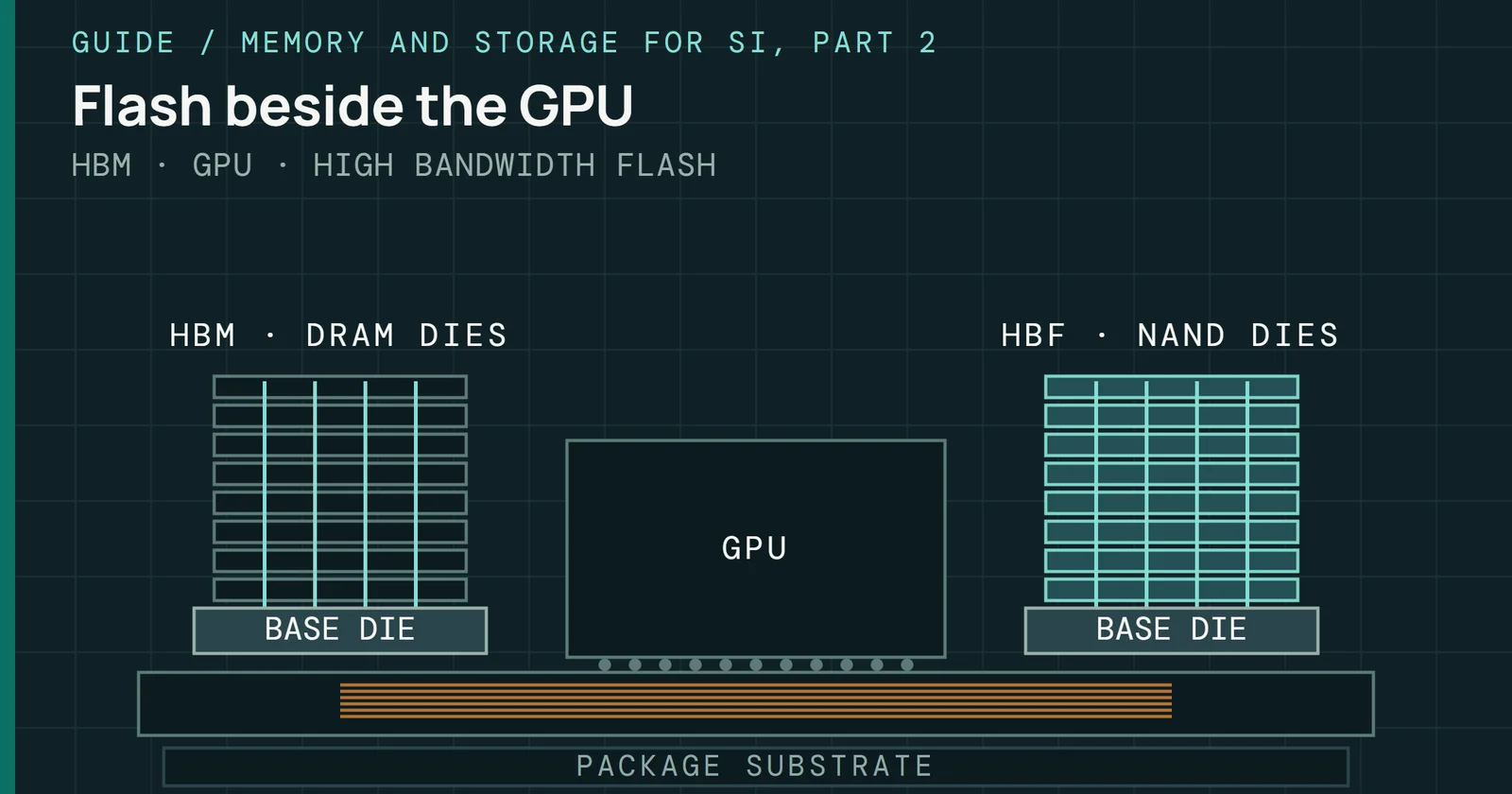
A standard SSD sits at the top of the figure and moves data to the host, which does the computing. Computational storage, in copper, moves a program to the data. High Bandwidth Flash leaves the NVMe path altogether and puts the flash beside the accelerator.
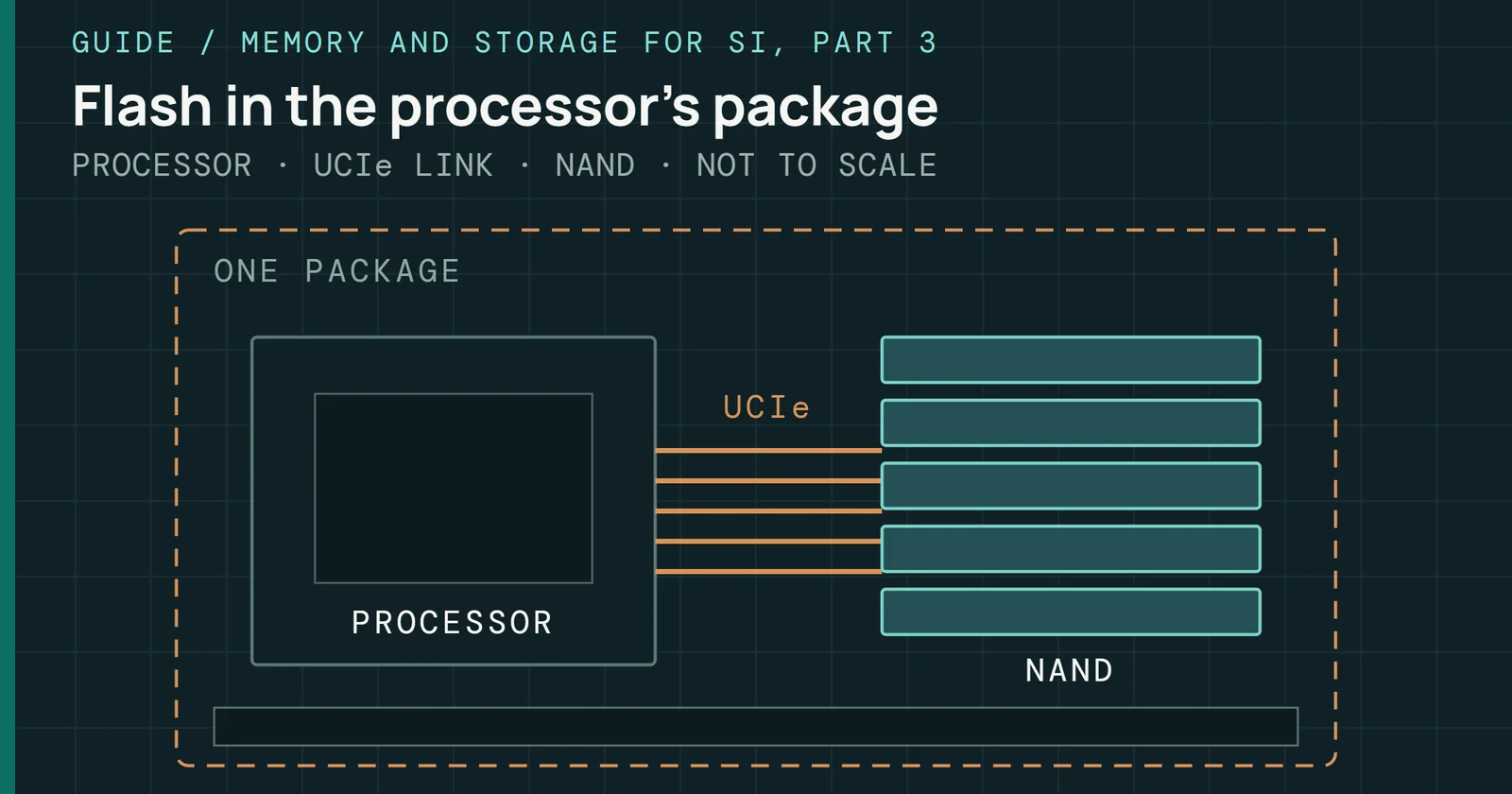
High Bandwidth Flash (HBF) is NAND stacked to sit beside an SI accelerator as a larger, slower tier next to HBM. It doesn’t sit behind an NVMe controller. As of October 2026, Sandisk and SK hynix released the first HBF specification through the Open Compute Project. It covers the host interface, electrical guidelines, reliability and packaging guidance for the die stack, and a software guide for reads and writes. By SK hynix’s own figures, stacks are 8-high or 16-high, hold up to 512GB, and come in three grades from 0.4 to 3.0TB/s over the Universal Chiplet Interconnect Express (UCIe) link. A published specification is not a part on sale. Sandisk’s 2025 announcement targeted first samples in the second half of 2026 and first SI-inference device samples in early 2027, and neither company’s August release names a product on sale. Beyond NAND’s guide on High Bandwidth Flash covers the specification, where HBF’s bandwidth comes from, and its limits in depth.
Computational storage moves processing to where the data lives. For large datasets where data movement dominates total processing time, offloading compression, encryption, filtering or search to the SSD cuts traffic across PCIe and reduces host CPU load. It is built for defined jobs. Blocks and Files reported in November 2022 that ScaleFlux’s CSD 3000 compresses and decompresses data transparently to the host, and a March 2024 report says the company supplied the CSD 2000 and CSD 3000 then. No later status was found. In those drives the engine does one fixed job. SNIA’s model is wider. An engine can be a CPU or an FPGA running configurable functions, and the table below lists that general-purpose case as research. NVMe’s Computational Programs command set standardizes how a host offloads a program. Beyond NAND covers other emerging memories, including Optane and phase-change memory.
More bits or more layers: the cost curve and the scaling limit
Cost per gigabyte follows how many good bits a wafer yields, and Part 4 owns the die density numbers. Wafer cost, yield and test cost go unpublished, so this section charts only what is public, which is bit density (bits stored per unit area). Layers were the main lever, and Part 4 covers the limits of a taller stack. Bits per cell is the other lever, and Figure 10.7 puts both on one scale.
More bits or more layers: the cost curve and the scaling limit
A 5-bit 3D die holds about 41 times the bits per area of planar
Bit density as a multiple of a planar 2-bit die; density printed above each bar
A planar 19nm die with two bits per cell held 64Gb on 112.8mm² (Kanda et al., JSSC 2013), so its density was 0.567Gb/mm². TechInsights’ densest triple-level cell (TLC) dies reach 8.47Gb/mm² at 128 layers, 11.01 at 176 and 15.03 at 232. That 232-layer die is about 26.5 times denser, so the same bits need about one twenty-sixth of the silicon. Intel reported (Khakifirooz et al., ISSCC 2023) a 192-layer die with five bits per cell at 23.3Gb/mm², about 41 times the planar die. Dividing out the bits per cell isolates the rest. A TLC die stores 1.5 times the bits per cell of the planar die, so the 232-layer die gets about 17.7 times from geometry. Geometry here means layer count, array efficiency and where the CMOS sits. Intel’s 5-bit cell gives 2.5 times from bits and about 16.4 times from geometry, a little less than the 232-layer die’s 17.7 times. Vendors and processes differ across these dies, so the split is only a reading aid. Part 4’s table spans TLC from 5.95Gb/mm² at 96 layers to 23.52 for SK hynix’s 321-layer die, and the top figure is about four times the bottom one.
Figure 10.7 charts area per bit and leaves price out. A denser die puts less silicon under each bit, but every added layer adds process work, so whether the bit gets cheaper depends on wafer cost and yield, which vendors don’t publish.
Each added bit doubles the number of states a cell must tell apart in the same voltage window, as Figure 10.8 shows, and Part 2 covers the progression from single-level to quad-level cells.
More bits or more layers: the cost curve and the scaling limit
Each added bit doubles the states in the same voltage window
States a cell must tell apart, by cell type
Figure 10.8’s copper bar is penta-level cell (PLC)PLC stores five bits per cell using thirty-two voltage levels, which packs more data into the same silicon but leaves very little margin between levels. flash, with five bits and 32 states. In Intel’s ISSCC 2023 paper on a 192-layer die with five bits per cell, a slide labels the step from four bits to five as 25%, and the conclusions claim 24% higher bit density than the best reported quad-level cell (QLC) densities. With 32 states to tell apart, guard bands tighten, raw error rates rise, and low-density parity-check (LDPC)LDPC is a code whose decoder passes confidence messages back and forth until the errors resolve. It corrects more errors than BCH, especially with soft input. error correction has more to correct. A January 2026 report says PLC had not gone commercial, so any endurance number for it is a guess. SK hynix’s split-cell design takes another route. It uses six states in each of two half-cells instead of 32 states in one cell, and pays for that in structural complexity.
Reports from January 2026 found no commercial PLC products on sale. Part 2 lists who has shown PLC work, and SK hynix presented 5-bit multi-site cell results at the International Electron Devices Meeting (IEDM) in December 2025. A research paper is not a production qualification, and none of these results shows the ECC and retention margin PLC needs working at volume. PLC remains a candidate for archive tiers that are rarely read, where capacity per die counts for more than endurance or speed. Timing is the open question. Will PLC reach volume production before taller stacks or bonded-die refinements give a better cost curveThe cost curve follows cost per gigabyte as die density rises, through more layers and more bits per cell. Public per-generation figures are scarce.? Industry roadmaps over the next couple of years will start to answer that.
Where one preprint says NAND goes next
In October 2026 a perspective paper called “The future of 3D NAND flash technology” was posted to arXiv. Most of its authors are university researchers at Georgia Tech and other schools, and one group is at Applied Materials. Two work in Samsung Electronics’ Advanced Device Research Laboratory, and Samsung supported the work in part. That makes it an academic and vendor-adjacent view of the road ahead. I read it as a framework and won’t treat it as proof that any of it works in a drive, and it isn’t a Samsung product announcement either. Everything in this section sits at the research end of Figure 10.11.
Its argument starts from the physics already covered in this series. With stacks heading toward kilolayer heights, the authors say process integration and lithography no longer set the pace of scaling. Charge spreading sideways inside the storage film, interference between neighboring cells, read disturb, the limit on current through a long polysilicon string, self-heating and threshold voltage spread each get worse with height. Its point is that no single one stops scaling. Together they eat the operating margin a little more each generation, and it calls this a margin-limited regime. Part 4 and Part 8 cover the same mechanisms from the die and the ECC side.
Figure 10.9 lists the two sets side by side, as the paper presents them.
Where one preprint says NAND goes next
One preprint lists four density levers and four use tiers
Both lists are the paper’s; it does not cross them in a table
Four ways to add density
Density now comes from four levers pulled at once, the paper says:
- Vertical scaling adds more layers, and Part 4 covers what a taller stack costs.
- Lateral scaling is finer partitioning of the array into blocks and sub-blocks in the plane, which fits more independently addressable units into the same die area.
- Logical scaling puts more bits in each cell, which raises capacity per layer and narrows the margin between states, as Figure 10.8 shows.
- Architectural scaling is where the peripheral circuits sit and how dies are joined, from circuits beside the array to circuits under it to separately made wafers that are bonded, as in the bonded interface section of Part 4.
Four tiers of use
On the other side, the paper splits demand into four tiers that want different things from the same NAND:
- Cold storage wants the most bits per die and long retention, and it tolerates modest endurance. The authors expect charge-trap flash to stay the choice here through the kilolayer transition.
- Active storage for SI training and inference wants sustained throughput and endurance. The paper suggests latency-sensitive inference buffers may run cells in an SLC-like mode, and it names ferroelectric NAND as a candidate for this tier.
- High bandwidth flash and big accelerator memory change the packaging and the access path and leave the cell alone. The first puts NAND dies and a controller behind a wide on-package interface. The second lets GPU threads start storage reads directly.
- Compute in memory uses the array itself to do multiply-accumulate work for neural-network inference, which needs uniform, well-separated conductance levels.
How I read the two lists together
The paper presents the vectors in one place and the tiers in another, and it doesn’t cross them in a table. Putting them side by side is my reading. Cold storage keeps leaning on the vertical and logical levers, because bit density is what it buys. Active storage leans the other way on the logical lever, trading bits per cell for speed and margin. The last two tiers are decided by the architectural lever and by system design more than by the cell. Their own summary is that future NAND will likely “evolve as a portfolio”, with no single successor to the charge-trap cell.
What this changes for a specification
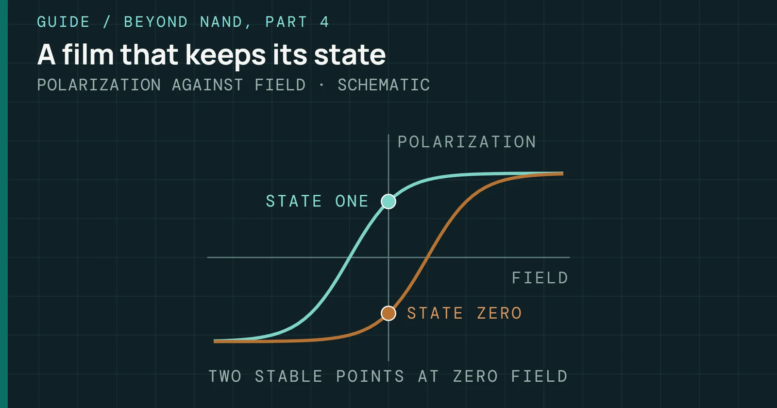
Nothing yet. The paper calls charge-trap flash the most mature 3D NAND technology and says ferroelectric NAND is particularly well suited to the active-storage and compute-in-memory tiers, though its demonstrated endurance, 10⁴ to 10⁶ program/erase cycles, falls short of enterprise targets. The authors suggest a hybrid, with ferroelectric cells for high-reliability blocks and charge-trap cells for bulk capacity, as the nearer-term route. No product like that is on sale, so it belongs with the other rows in the bottom stage. If a vendor cites this paper, ask which of the four levers or tiers the claim is about, and whether the result is a lab demonstration or a qualified part.
In the field: telling products from roadmap
A vendor deck says a drive supports a feature. Whether it does depends on the product, the host and the platform, and the answer lives in logs and labels. Figure 10.10 orders the two questions that decide it.
In the field: telling products from roadmap
Two questions sort a claim: can you buy it, can you run it
Product first, then host and platform
The first question separates a part you can buy from a specification or a sample. The second separates a part that works in your stack from one that needs host software or a platform you don’t run, and four checks answer both.
Read the device, not the press release
A connector that looks identical can hide an NVMe 1.4, 2.0 or 2.4 device, and ZNS, KV and Computational Programs are optional command sets (Part 1 lists them). Whether a given drive implements one is a firmware question, so read Identify. For Streams, the Optional Admin Command Support (OACS) field reports Directives and a Directive Receive Identify command confirms them, and data sheets often omit Streams or FDP support, so confirm it during qualification (Part 6).
Read the bay, not the connector
An E3.S bay can hold a CXL memory module, and Identify will not describe it. Read the JEDEC module label for media type, CXL revision, capacity and connector width (Part 1). A platform CPU that doesn’t speak CXL won’t bring the module up as memory.
Check host support before blaming the drive
A drive that supports FDP hints but receives untagged writes gains nothing, and a ZNS drive needs a zone-aware stack. Both are host work, so a missing benefit is often a missing host feature.
Separate a model shift from wear
If learned models reach drives on sale, a drive’s behavior may change when the model shifts, even with no wear and no hardware fault behind it. Telling the two apart requires knowing what the adaptive system optimizes and what NAND physics predicts at that wear level. Compare the drive with its cohort at equal wear, using the SMART fields that Part 8 owns. Tools measure the outcome. ioTraX covers real-time I/O behavior, TriageIO covers fleet-level SMART telemetry, and IOSpeX covers error log extraction. Knowledge of the physics and firmware from this series says what the outcome means.
What to specify today and what to watch
For a product manager or field engineer making storage decisions in 2026, the relevant question is what is production-ready for this deployment. Figure 10.11 sorts the directions in this part into four stages by how far each is from a purchase order, as of October 2026.
What to specify today and what to watch
Four stages separate what is on sale from what is still a roadmap
As of October 2026, from purchasable to research
The top stage is where a specification can name a feature today. At the bottom stage it should not. Below, a table adds what each direction depends on and when to expect it.
| Technology | Status | Practical timeframe (editorial estimate) | Ecosystem dependency |
|---|---|---|---|
| Workload-adaptive GC and classification | Vendor-described, consumer and enterprise firmware | Now | None |
| Flexible Data Placement | Production, hyperscale | Now | Host placement hints (RocksDB, Ceph, application layer) |
| ZNS drives | Data sheet and reseller listing | Reseller-listed for drives, several years out for broad enterprise | Zone-aware host software (f2fs, btrfs zoned mode, RocksDB through ZenFS) |
| KV command set drives | Prototype (Samsung, 2019) | Several years out for broad enterprise | KV-native application or database layer |
| CXL 1.1 memory expansion | Production, specific platforms | Now on Emerald Rapids or Genoa servers or later | Intel 5th Gen Xeon or AMD EPYC 4th Gen, or later |
| CXL 2.0 memory pooling | Type 3 on Xeon 6; pooling silicon sampling with hyperscalers | Now for expansion, a few years out for broad pooling | Xeon 6 or later, CXL switch fabric |
| PCIe 6.0 SSDs (data center) | Production, enterprise | Now from Micron and Samsung; a Tom’s Hardware guide of October 6, 2026 lists no PCIe 6.0 consumer M.2 drive | New controller silicon, PAM4 and FEC, EDSFF connector |
| Computational storage for fixed jobs | ScaleFlux compression drives, as of March 2024 | Now for fixed jobs; no later status found | Workload-specific integration |
| High Bandwidth Flash | Specification published, samples targeted for 2026 and 2027 | No product on sale | Accelerator and package ecosystem |
| Per-drive learned models beyond retry tables | Research, not publicly documented in drives on sale | No firm timeline | Controller silicon with inference capability |
| On-device training | Research or early qualification | Several years out | Silicon area budget, validation framework |
| CXL 3.x fabric topology | Switches demonstrated, no platform confirmed on sale | Several years out | Full platform and switch ecosystem |
| General-purpose computational storage | Research, NVMe command set ratified | No firm timeline | Host software ecosystem maturity |
| Penta-level cell flash | Research and demonstration | No firm timeline | Error correction and retention margin |
What does not change
Charge still sets a threshold voltage, pages still can’t be overwritten in place, blocks still erase whole, and error correction still absorbs what the cells get wrong. Smarter firmware, a zoned namespace or a CXL bay changes the workload the NAND sees and where the bookkeeping happens, not those limits. A feature that can’t be traced to one of those layers needs checking before anyone calls it a fact.
The dated items to watch are Marvell’s Bravera SC6 sampling to partners in Q4 2026, Phison’s X3 sampling in December 2026 and shipping in volume in mid-2027, AMD’s Venice SP7 platforms in Q4 2026, Sandisk’s High Bandwidth Flash samples targeted for the second half of 2026, and the August 2027 NVMe release that plans to obsolete Predictable Latency Mode and NVM Sets. Each is a forecast, and a date that passes without the matching product on sale is the signal to note.
What does not change
The future of flash rests on every part below it.
The last part, resting on the nine below it.
This is the end of the series. For the memories built to sit beside NAND, read Beyond NAND and its guide on High Bandwidth Flash. Where each family sits closes that series and places them by job. To watch the mechanisms from this series move, open the labs.
Sources
Primary is the original paper, standard or datasheet. Secondary is a review, a vendor summary or a news report. Measured is my own test data.
Show all 48 sources, 22 primary
- PrimaryA 19 nm 112.8 mm2 64 Gb Multi-Level Flash Memory With 400 Mbit/sec/pin 1.8 V Toggle Mode InterfaceIEEE Journal of Solid-State Circuits, 2013
- PrimaryA 1.33-Tb 4-Bit/Cell 3-D Flash Memory on a 96-Word-Line-Layer TechnologyIEEE Journal of Solid-State Circuits, 2020
- PrimaryNVM Express: SpecificationsNVM Express - scalable, efficient, and industry standard, 2020
- PrimaryZNS+: Advanced Zoned Namespace Interface for Supporting In-Storage Zone CompactionUSENIX OSDI 2021
- PrimaryA 1.67Tb, 5b/Cell Flash Memory Fabricated in 192-Layer Floating Gate 3D-NAND Technology and Featuring a 23.3Gb/mm2 Bit DensityISSCC, 2023
- PrimaryXConn Technologies Releases Early Production Silicon Samples of 'Apollo' CXL 2.0 Switch at MemCon 2024prnewswire.com, 2024
- PrimaryCXL Consortium Releases the Compute Express Link 4.0 SpecificationCXL Consortium, 2025
- PrimaryAMD EPYC 9005 Series Processors data sheetAMD
- PrimaryChanges in NVM Express Specifications
- PrimaryChanges in NVM Express Specifications, August 2026NVM Express
- PrimaryComparison: Latest 3D NAND Products from YMTC, Samsung, SK hynix and Micron (TechInsights)
- PrimaryComputational Programs Command Set SpecificationNVM Express
- PrimaryCXL Consortium releases the Compute Express Link 4.0 specificationCXL Consortium
- PrimaryKey Value Command Set SpecificationNVM Express
- PrimaryMicron 9650 SSD, the world's first PCIe® Gen6 SSD, reaches a new shipping milestone!Micron Technology
- PrimaryNVM Express Base Specification, Revision 1.4cNVM Express
- PrimaryNVM Express specificationsNVM Express
- PrimaryOverviewzonedstorage.io
- PrimaryPCI-SIG FAQ: PCI Express 6.0PCI-SIG
- PrimarySNIA Computational Storage Architecture and Programming Model 1.0SNIA
- PrimaryThe PCIe 7.0 Specification, Version 1.0 is Now Available to MembersPCI-SIG
- PrimaryZNS: Avoiding the Block Interface Tax for Flash-based SSDs
- SecondaryPAM4 Basics: Modulation, Signaling and EncodingEDN, 2016
- SecondaryMicrochip Makes ML, AI Advances with Flashtec SSD ControllerEE Asia, 2021
- SecondaryScaleFlux makes go-faster computational storage SoCblocksandfiles, 2024
- SecondaryFMS 2025 CXL Demos - Compute Express LinkCompute Express Link -, 2025
- SecondaryAMD 6th Gen EPYC Venice: 256 cores, 1.6TB/s, and the first PCIe Gen 6 server CPUStorageReview, 2026
- SecondaryBest SSDs 2026: From blazing-fast M.2 NVMe down to budget SATATom's Hardware, 2026
- SecondarySK hynix developing split-cell 5-bit flashBlocks & Files, 2026
- SecondaryThe future of 3D NAND flash technology (arXiv 2610.06363)arXiv, 2026
- SecondaryAMD 6th Gen EPYC Venice: 256 Cores, 1.6TB/s, and the First PCIe Gen 6 Server CPUStorageReview.com
- SecondaryAs computational storage gets more buzz, ScaleFlux talks up latest CSDsBlocks and Files
- SecondaryAstera Labs Bolsters Leo Smart Memory Controller Family for Agentic AI and General-Purpose Cloud WorkloadsASTERA LABS, INC.
- SecondaryAstera Labs Leo CXL Smart Memory Controllers on Microsoft Azure M-series Virtual Machines Overcome the Memory WallASTERA LABS, INC.
- SecondaryCXL is finally coming in 2025ServeTheHome
- SecondaryCXL is Finally Coming in 2025 (ServeTheHome)ServeTheHome
- SecondaryFlexible data placementLWN.net
- SecondaryGen5 vs Gen6 PCIe: what do you need to know?Quarch Technology
- SecondaryHow to choose an interconnect for PCIe 6.0 high-speed systemsSignal Integrity Journal
- SecondaryHyperscalers embrace Flexible Data Placement (FDP) to increase performance and lower TCOSamsung Semiconductor
- SecondaryPCI-SIG releases PCIe 7.0 specification to support the bandwidth demands of AI at 128.0 GT/sSignal Integrity Journal
- SecondaryPhison shows PCIe 6.0 X3 SSD controller with 28 GB/s of bandwidth and 6.8 million IOPSTom's Hardware
- SecondarySamsung's open source key:value SSD is a game-changer for unstructured appsBlocks and Files
- SecondarySK hynix H25GTD0 321-layer V9 1 Tb TLC 3D NAND process flow analysis (TechInsights)
- SecondarySK hynix unveils 5-bit NAND that splits cells, delivers 20x faster readsTrendForce
- SecondaryThe current state of PCIe 6.0 SSDs and controllersTom's Hardware
- SecondaryUltrastar DC ZN540 data sheetWestern Digital
- SecondaryWestern Digital Ultrastar DC ZN540 NVMe SSDAdvanced HPC